Federal Airborne LiDAR Data Acquisition Guideline

Version 3.1, 2022

Natural Resources Canada, General Information Product 117e.
Natural Resources Canada, Public Safety Canada.
© His Majesty the King in Right of Canada, as represented by the Minister of Natural Resources, 2022.
For information regarding reproduction rights, contact Natural Resources Canada at copyright-droitdauteur@nrcan-rncan.gc.ca.

Table of Contents

List of abbreviations and acronyms

ANPD: Aggregate Nominal Pulse Density
ANPS: Aggregate Nominal Pulse Spacing
AOI: Area of Interest
ASPRS: American Society of Photogrammetry and Remote Sensing
CHA: Calculated Horizontal Accuracy
CCMEO: Canada Centre for Mapping and Earth Observation
CGG2013: Canadian Geoid 2013
CGVD: Canadian Geodetic Vertical Datum
CORS: Continuously Operating Reference Stations
CQL: Canadian Quality Level
CSRS: Canadian Spatial Reference System
DCAOI: Data collection Area of Interest
DEM: Digital Elevation Model
DSM: Digital Surface Model
DTM: Digital Terrain Model
EPSG: European Petroleum Survey Group
ESRI: Environmental Systems Research Institute
GLONASS: Globalnaya Navigazionnaya Sputnikovaya Sistema
GNSS: Global Navigation Satellite System
GPS: Global Position System
GRS80: Geodetic Reference System 1980
IMU: Inertial Measurement Unit
INS: Inertial Navigation System
ISO: International Standard Organization
LAS: LASer file format exchange
LAZ: LASzip
LiDAR: Light Detection and Ranging
NIR: Near Infrared
NPD: Nominal Pulse Density
NPS: Nominal Pulse Spacing
NRCan: Natural Resources Canada
NTS: National Topographic System
NVA: Non-Vegetation Vertical Assessment
OGC: Open Geospatial Consortium
PDOP: Position Dilution of Precision
PLS: Pulse(s)
PPP: Precise Point Positioning
RMSE_X: Horizontal Root Mean Square Error in the x direction (easting)
RMSE_Y: Horizontal Root Mean Square Error in the y direction (northing)
RMSE_R: Horizontal Root Mean Square Error in the radial direction (includes both x and y directions)
RMSE_Z: Vertical Root Mean Square Error in the z direction (elevation)
RMSD_Z: Vertical Root Mean Square Difference in the z direction (elevation)
RTK: Real Time Kinematic
SBET: Smooth Best Estimate Trajectory
TIN: Triangular Irregular Network
USGS: United States Geological Survey
UTM: Universal Transverse Mercator
VVA: Vegetation Vertical Assessment
WKT: Well Known Text
XML: eXtensible Markup Language

1.0 Introduction and purpose

Development of this document has been coordinated by the Canada Centre for Mapping and Earth Observation (CCMEO) within Natural Resources Canada (NRCan) in response to the needs of the geospatial community and the government for a national guideline for acquisition of airborne LiDAR data. A key strategy of the CCMEO is to improve the national elevation data set through consistent application of airborne LiDAR technology. LiDAR has extensively been adopted across Canada by municipalities, provinces, territories and federal government departments as the main technology for acquiring high precision elevation data. The intention of this document is to provide the specifications to lead towards consistency in airborne LiDAR data acquisition across all levels of government in Canada, as well as to improve international cooperation with the United States along areas of cross-border data collection.

The process for developing the guideline has involved consultation with government, industry and academia, as well as a review of international best practices to provide a broad perspective for establishing the guideline. The federal guideline addresses many complex considerations including data acquisition, processing, validation, and deliverables, with the focus on developing accurate elevation data. The emphasis of the guideline is on data quality and accuracy requirements, while allowing for innovation and future technological advancements. It is the aim of the guideline to accommodate project-specific requirements, and there are cases where the suggested LiDAR acquisition specifications may be relaxed or modified due to factors such as project data requirements and financial considerations. The intent of this guideline is to set quality levels and good practices to achieve the various federal government needs. The guideline also contains supplemental recommendations for LiDAR acquisition in specific application areas, including forestry, flood mapping, mapping of high relief areas, and urban infrastructure.

LiDAR acquisition is an industry heavily reliant on cutting edge technology and is therefore seeing constant improvements in the technological components used in surveys, as well as software and methods used in LiDAR analysis. This document is reflective of the best practices in LiDAR acquisition at the time of the document release. NRCan intends to update this document periodically as the industry develops.

2.0 Note on terminology

This guideline contains numerous references to industry specific terms that may vary in other application areas or differ from other guidelines or specifications. For example, in the LiDAR community, bare earth DEM is commonly used to represent ground surface terrain. In this guideline, DTM is used in alignment with the High Resolution Digital Elevation Model (HRDEM) – CanElevation Series -Product Specification (PDF, 1.2 mb). DTM is considered equivalent to bare earth DEM. In addition, the term ‘pulse’ is used to represent the transmitted and received laser electromagnetic energy, while ‘point data’ represents pulse data that has been post processed and classified into point cloud. A glossary included in this document provides term definitions in the context of the present guideline.

3.0 Target audience

This document is part of the Federal Flood Mapping Guidelines Series and is to be used as a resource for the acquisition of base elevation data from airborne LiDAR data undertaken across Canada. This guideline aims to provide advice to federal, provincial and territorial departments, whose responsibility is to provide technical guidance to their implementing bodies, as well as individuals and organizations in Canada that need to understand and plan for airborne LiDAR data acquisition. Users of this guideline may include department managers, project coordinators, geomatics experts, water resource engineers, and planners both within and outside of government. The document assumes that users have basic understanding of LiDAR technology and data, including terminology and data structure.

Some provinces and territories have already developed their own guidelines and specifications for airborne LiDAR data acquisition. Hence, this guideline is intended as a basis to further harmonize requirements for acquiring LiDAR data across Canada.

4.0 Guideline structure

The guideline has been organized based on a workflow structure involving planning, collection, processing, data validation and expected deliverables of airborne LiDAR data in the context of a Canadian landscape. Information on forest, urban infrastructure, flood and high relief mapping applications has been provided in the appendices section of the guideline. Appendices represent current best practice for collection of airborne LiDAR data. Recommended data and collection parameters are provided. In addition, an annex is also included for addressing contract related items for project data collections. The structure of the guideline is referenced by categories as listed below.

Planning
Acquisition
Data Processing
Validation
Deliverables

5.0 Summary requirements

Requirements for the acquisition of airborne LiDAR data are summarized in Table 1 and presented in the form of generic formulas. "Canadian Quality Level 1" (CQL1) is the minimum requirement for airborne LiDAR data acquisition in Canada, as well as to support the Government of Canada's National Elevation Data Strategy. This strategy aims to provide Canadians with a detailed three-dimensional representation of the territory and to offer standardized products that allow consistent analyses across the country.

Some areas of application require more accurate and/or denser LiDAR data than CQL1. For these LiDAR acquisitions, the generic formulas presented in Table 1 can be used to establish the requirements. Examples of values to be used in the formula (replacing the terms ANPD, RMSE_z and RMSE_R) are provided in the appendixes of this document for various areas of application.

Section 6 provides further details on project planning, data validation and deliverables. There are also recommendations, assumptions and considerations. In the same way as for Section 5, the tables in Section 6 contain generic formulas and values for CQL1. Users are encouraged to read this entire document to learn more about the requirements.

**Table 1: Requirements summary**
Requirements	Generic specifications	Example for the Canadian Quality Level 1 (CQL1)	Category
Aggregate Nominal Pulse Density (ANPD)	≥ ANPD	≥ 2 pulses/m²	Acquisition
Aggregate Nominal Pulse Spacing (ANPS)	≤ $\frac{1}{\sqrt{ANPD}}$	≤ $\frac{1}{\sqrt{2}} \to 0.71 m$	Acquisition
Non-vegetated Vertical Accuracy (NVA)
Vertical Root Mean Square Error (RMSE_Z)	≤ RMSE_Z	≤ 10.0 cm	Acquisition
Vertical Accuracy – 95% confidence level	≤ 1.96 x RMSE_Z	≤ 1.96 x 10 → 19.6 cm	Acquisition
Vegetated Vertical Accuracy (VVA) – 95th percentile	≤ 3 x RMSE_Z	≤ 3 x 10 → 30 cm	Acquisition
Fundamental Horizontal Accuracy (FHA)
Horizontal Root Mean Square Error (RMSE_R)	≤ RMSE_R	≤ 35.1 cm	Acquisition
Horizontal Accuracy – 95% confidence level	≤ 1.7308 x RMSE_R	≤ 1.7308 x 35.1 → 60.0 cm	Acquisition
Calculated Horizontal Accuracy (CHA)	≤ RMSE_R	≤ 35.1 cm	Acquisition
Relative Vertical Accuracy
Intraswath (smooth surface repeatability) - RMSD_Z	≤ 0.6 x RMSE_Z	≤ 0.6 x 10 → 6 cm	Validation
Interswath (swath overlap difference) – RMSD_Z	≤ 0.8 x RMSE_Z	≤ 0.8 x 10 → 8 cm	Validation
Interswath (swath overlap difference) – Maximum difference	≤ 1.6 x RMSE_Z	≤ 1.6 x 10 → 16 cm	Validation
Horizontal Datum	Variable	NAD83 CSRS epoch 2010	Acquisition
Vertical Datum	Variable	CGVD2013	Acquisition
Geoid Model	Variable	CGG2013	Acquisition
Map Projection	Variable	Universal Transverse Mercator	Acquisition
Minimum Swath Overlap	15 %	15 %	Acquisition
Pulse Returns	Minimum 2 returns (First and Last). Intermediate is optional.	Minimum 2 returns (First and Last). Intermediate is optional.	Acquisition
Classification	Variable	1 – Processed but unclassified 2 – Ground 7 – Low points (noise) 9 – Water 1 7 – Bridge decks 18 – High noise	Processing

6.0 GUIDELINE

6.1 Project planning

Prior to airborne LiDAR data collection, vendors will undertake activities to design an acquisition plan and establish a processing approach to meet the specification as outlined in this document. Key planning tasks are identified in the following sections and will form part of the project deliverables. The following sections outline the type of information that will be assembled into a Project Report.

6.1.1 Project method

Description

The vendor is required to provide details on the methodology selected meets the technical requirements of the specifications. The project methodology must be described in a project planning report to be submitted in advance of the data collection.

Requirements

**Table 2: Project method requirements.**
Name	Description	Category
Flight Planning	Details on flight coverage, flight line location, overlap, calibration flights, tie lines, including visual references such as maps and images. A detail work flow with quality control measures and survey work will be provided.	Planning
Survey Control	Proposed surveying control to support airborne GNSS and any ground validation will be identified with details including base stations (bg-info or passive) to be used, along with the reference information on the position control.	Planning
Ground Truthing	Details on planned ground validation and in-situ measurements, including location, and propose method for collecting ground survey data.	Planning
Data Processing	Details on the planned data processing including software, methods, filtering, any ancillary data to be used in data processing. A schematic work flow diagram showing the data processing steps and the quality control procedures incorporated in the processing will be included.	Planning
Quality Control	Data validation method, check for classification, accuracy verification, data voids, and other data checks. Information should include frequency and quantity sampled	Planning
Schedule	Planned schedule for airborne collection and ground truthing activities.	Planning

Considerations, Limitations and Assumptions

Any deviation from the project methodology will be provided to the contracting authority in advance of the data collection for review and approval.

6.1.2 Instrumentation

Description

A document is required that provides details on the airborne and ground survey equipment proposed for the project. The document should include specifications (including manufacturer, model and year) of the LiDAR sensor, the GNSS system used in the aircraft, the IMU sensor, and the ground survey instrumentation. The document should also include details regarding the calibration of the sensors including date of the last calibration. The document should be provided as part of the project deliverables.

Requirements

**Table 3: Instrumentation requirements.**
Name	Description	Category
Sensor Instrument	Details of the specific LiDAR sensor will be provided including manufacturer, year, model, ownership, most current calibration with date. A copy of the most current manufacturer’s calibration for the complete system including laser, IMU, and GNSS system used maybe requested and upon request must be provided. Any sensor changes, failure or replacement prior or during the data collecting is required to be reported.	Planning
GNSS	The type of position sensors used in the acquisition (ground and airborne) is documented. Details to be provided include the manufacturer, year, and model. Any reference network information (bg-info or passive) including number, location monuments, reference statement and published coordinates must be provided.	Planning
IMU	Provide details on the proposed IMU for the data collection including manufacturer, year, and model.	Planning

Considerations, Limitations and Assumptions

Any deviations from the proposed instrumentation must be communicated to the contracting authority for approval in advance of the data collection. The alternative instrumentation must be equal or better than planned sensors. The contracting authority may accept or reject proposed changes.

6.1.3 Data Collection Planning

Description

The minimum requirements for planning a collection of airborne LiDAR data are provided below.

Requirements

**Table 4: Data collection planning requirements.**
Name	Description	Category
Area of Interest (AOI)	A project area of interest is defined in the form of enclosed geographic boundaries using the coordinate system as identified in this guideline.	Planning
Data Collection Area of Interest (DCAOI)	A buffer of 100 metres is uniformly applied to the AOI and represents the actual data collection coverage. Data collected in the buffer area is to be submitted as part of the deliverables and must be collected to the same requirements as the data within the AOI.	Planning
Discrete Returns	The system used in the collection must be capable of collecting multiple discrete returns per pulse. At minimum, first and last returns are required. Intermediate returns are optional. Waveform data is optional.	Planning
Intensity	The intensity for each discrete return will be recorded and stored and as a 16-bit normalized value. A linear scaling will be applied as defined in ASPRS LAS 1.4 R15.	Planning
Swath Overlap	A minimum of 15% swath overlap is required for a CQL1 acquisition. However, the swath overlap requested by the contracting authority in the acquisition contract can be higher.	Planning

Considerations, Limitations and Assumptions

Airborne LiDAR data acquisition is dependent on using a reference control data source to precisely position the LiDAR pulses returns from the land surface. The reference control data for mapping the position of the pulse return use a range of global navigation satellite systems (GNSS). These systems include different constellations such as GPS, GLONASS, QZSS, Galileo or BeiDOU. However, the application of GNSS for positioning is affected by satellite geometry and solar flare which creates instability in the ionosphere. Therefore, it is recommended that a Position Dilution of Precision (PDOP) be less than 3, that a minimum of 7 satellites be in view, and that solar weather be checked prior and during data collection. A Single Ground base station for correcting GNSS signals should typically be within 25-35 km of field collection. Depending on the size and configuration of the DCAOI, two or more ground base control stations is recommended with baselines longer than 35km. bg-info control GNSS correction for RTK that use Continuous Operating Reference Stations (CORS) for real time correction or post processing such as Canadian Geodetic Survey PPP is permissible. The use of satellite-derived PPP corrections is also permissible. The vendor must provide information on the positional method and ensure that the proposed solution meets the accuracy requirements of this guideline. Further information may be found in the Guidelines for RTK/RTN GNSS Surveying in Canada (2013).

Cross-tie lines are flight lines acquired perpendicular to the planned data acquisition flight lines. Cross-tie lines provide data to support accuracy validation and can be used to support adjustment of data such as in periods of unexpected poor PDOP. It is strongly recommended that cross-tile lines be collected to support data quality assessment and validation.
The requirement for swath overlap is a minimum of 15% for a CQL1 acquisition to support quality assessment between adjacent swaths and to minimize potential data gaps. Actual overlapping swath used in the collection is at the discretion of the data collector to ensure the absence of data gaps in the useable portion of the swath (typically centre 95% of the swath width) and that the required data density is met.
The scan angle used for airborne LiDAR data collection typically ranges from ±15 to ±30 degrees. Higher scan angles are discouraged as they result in increased footprint size thereby reducing pulse energy at the edges, increasing positional errors and scattering off the sides of vertical structures. In addition, when collection over undulating and/or high relief terrains, higher scan angles should also be discouraged. Best practice typical angles are between ±20 to ±25 degrees. The selection of a scan angle should consider vertical and horizontal accuracy requirements across the swath as well as per the project objective.

6.2 Data Collection

This section provides details on how to meet airborne LiDAR data acquisition requirements.

6.2.1 Conditions

Description

LiDAR data collection is affected by surface and atmospheric conditions which impact the quality and quantity of LiDAR pulse returns. This section describes the minimum requirements for airborne LiDAR acquisition with respect to the atmospheric, surface and other conditions.

Requirements

**Table 5: Data collection conditions requirements.**
Name	Description	Category
Atmospheric	Collection should not take place during rain, snowfall, smoke or fog. No haze or clouds should be present between the aircraft and the ground.	Acquisition
Surface	Surface should be free from extensive flooding or inundation, snow cover and ice buildup on shoreline or land areas. Dry land surface condition is required. Frost is acceptable.	Acquisition
Tides	Areas affected by tides should be collected within 2 hours of the low tide. Low tide is time when the tide will be at its lowest point for given place and time the collection will take place.	Acquisition
Survey	Monitoring and recording of Global Navigation Satellite System conditions for Positional Dilution of Precision and solar activities during acquisition is required.	Acquisition
Temporal	Aside from the low tide requirement, there is no restriction on the time of day for LiDAR acquisition. Data may be acquired during day or night, provided data collection is compliant within any regulatory or legal conditions, and safety requirements are given paramount attention.	Acquisition

Considerations, Limitations and Assumptions

The collection of LiDAR data is encouraged during river low flow (baseflow) conditions to maximize coverage of river banks and floodplains.
At the discretion of the contract authority, the snow-free surface requirement may be waived for areas where there are permanent snowfields or glaciers.
Except for specialized data collection projects focusing on vegetation (for example, forest biomass studies), leaf-off is a preferred vegetation condition, since it increases penetration to the ground and results in higher quality bare-earth surface (see Annex A). Leaf-on collection may be acceptable if the vendor collection method can demonstrate sufficient ground penetration to achieve accurate and reliable bare-earth surface that meet accuracy requirements. The contract authority will work with the vendor to determine acceptable vegetation conditions for LiDAR acquisition in the DCAOI.
Very light non-drifting snow cover (less than 1cm) may be permissible at the discretion of the contracting authority.

6.2.2 Collection Pulse Density

Description

LiDAR pulse density and spacing for DCAOI is defined in this guideline as an aggregate nominal pulse density (ANPD) and aggregate nominal pulse spacing (ANPS). The aggregate pulse density/spacing is referred to as an overall pulse density/spacing whereby a swath may overlap other swaths completely, partially, or not at all. An overlapping swaths condition is achieved when a portion of the swath is covered with an adjacent flight line, flown on top of an existing swath with a single sensor, or acquired by two independent sensors using separate IMU’s, with separate boresights on the same aircraft. A dual channel system using single Inertial Navigation System (INS) and boresight is considered to be acquiring single swath data. In swaths where a portion of the swath has no overlap then ANPD/ANPS is equivalent to Nominal Pulse Density and Nominal Pulse Spacing (NPD/NPS). See glossary for further definitions.

Requirements

**Table 6: Pulse density requirements**
Name	Description	Category
Aggregate Nominal Pulse Density (ANPD)	≥ ANPD (pls/m²) evaluated with first pulse returns across DCAOI	Acquisition
Aggregate Nominal Pulse Spacing (ANPS)	≤ $\frac{1}{\sqrt{ANPD}}$	Acquisition
Laser Returns	Pulse data collection is based on laser pulse echo returns measured at the receiving sensor. At a minimum, first and last returns are required and intermediate returns are optional.	Acquisition

Note: For the CQL1, replace ANPD by 2. For areas of application requiring denser LiDAR data than CQL1, use the suggested ANPD values in the appendixes of the present Guideline.

Considerations, Limitations and Assumptions

ANPD and ANPS in this Guideline document refers to the net overall pulse density and pulse spacing from multiple independent sensors or multiple overlapping swaths. For single swath, ANPD and ANPS equal, respectively, to NPD and NPS.
An intermediate pulse can provide addition information for applications involving forest/trees, transmission/distribution wires and buildings.

6.2.3 Data Collection Accuracy

Description

This section covers requirements for absolute and relative vertical and horizontal accuracy of LiDAR acquisition.

Requirements

**Table 7: Data collection accuracy requirements**
Name	Description	Category
Non-vegetated Vertical Accuracy (NVA)
Vertical Root Mean Square Error (RMSE_Z)	≤ RMSE_Z	Acquisition
Vertical Accuracy – 95% confidence level (1.96 * RMSE_Z)	≤ 1.96 x RMSE_Z	Acquisition
Vegetated Vertical Accuracy (VVA) - 95th percentile	≤ 3 x RMSE_Z	Acquisition
Fundamental Horizontal Accuracy (FHA)
Horizontal Root Mean Square Error (RMSE_R)	≤ RMSE_R	Acquisition
Horizontal Accuracy – 95% confidence level	≤ 1.7308 x RMSE_R	Acquisition
Calculated Horizontal Accuracy (CHA)	≤ RMSE_R	Acquisition
Relative Vertical Accuracy
Intraswath (smooth hard surface repeatability) - RMSD_Z	≤ 0.6 x RMSE_Z	Acquisition
Interswath (swath overlap difference – RMSD_Z)	≤ 0.8 x RMSE_Z	Acquisition
Interswath (swath overlap difference) – Maximum difference	≤ 1.6 x RMSE_Z	Acquisition

Note: for the CQL1, replace RMSE_Z by 10 cm and RMSE_R by 35.1 cm. For areas of application requiring more accurate LiDAR data than CQL1, use the suggested RMSE_Z and RMSE_R values in the appendixes of the present Guideline.

The Calculated Horizontal Accuracy (CHA) - Horizontal accuracy is influenced by GNSS positional errors, the angular errors arising from the IMU used and the flight altitude. A calculated horizontal accuracy will be derived using LiDAR Horizontal Error (RMSE_r) in ASPRS 2014 Positional Accuracy Standards for Digital Geospatial Data in Section 7.5. The formula is as follows:

$LiDAR Horizontal Error (RMSEr) = \sqrt{(GNSS positional error)^2 + (tan ⁡ (IMU error) / 0.55894170 x flying altitude)^2}$

More details on the usage of the formula are given here: Mapping Matters

Considerations, Limitations and Assumptions

The accuracy assessment should be conducted within the geometrically usable portion of the swath (typically the centre 95% of the swath width). The horizontal and vertical accuracy of the ground check points must be three times more accurate than the LiDAR and always better than 5 cm (95%). See section 6.4.1 for more details.
The relative vertical accuracy is used to examine geometric stability across all portions of the swath for data consistency. The overlap area can be considered as a measure of geometric alignment of two overlapping swaths with respect to positional shifts and vertical alignment. In addition, relative accuracy is a measure within the swath to detect any anomalous pulse data potentially due to laser issues and sensor related anomalies. The assessment is to be done at multiple locations throughout the DCAOI. See Data Validation section for more details.

6.3 Data Processing and Management

6.3.1 Data File Format

Description

Collected LiDAR point cloud data should be stored in the ASPRS LASer File Exchange format (LAS). For bulk storage of data, LAS files can be compressed into the lossless LAZ (LAS zip) format.

Requirements

**Table 8: Data file format requirements.**
Name	Description	Category
Standard	ASPRS LAS 1.4 – R15 will be used for storing LiDAR point cloud data. LAS 1.4 moves to 64-bit file structure.	Data Processing
Content	The Public Header information is to be completed.	Data Processing
Pulse Data Record	Record Formats 6, 7, 8, 9, or 10 are to be used for discrete pulse data. The format values depend if colour information is added and or wave packets are added to the LAS record structure.	Data Processing
Overlap and Overage	Overage pulses in the swath overlap region (i.e. points not part of the tenderloin) shall be identified as using overlap bit 3 flag as described in Table 16 in LAS 1.4 – R15 specification for Record Format 6. Applying a point classification field in any way for overage/overlap is not permissible. See definition of overage in glossary.	Data Processing
Withheld Pulses	Withheld pulses due to noise, erroneous data points, and geometrically unreliable points should be retained using classification bit 2 as per Table 16 in LAS 1.4 – R15 specification.	Data Processing
Swath identification	A unique file identifier (File ID) for individual flight swaths must be applied prior to data processing and available to identify each swath to source as identified in LAS 1.4 specification. Each point within the swath must also be assigned a point source identifier (Point Source ID) that equals the unique file identifier. The unique file and point identifier must be persistent and preserved through the data processing steps.	Data Processing
Georeference	A correct and properly formatted geo-reference must be present in all LAS file headers. Open Geospatial Consortium (OGC)’s Well-Known Text (WKT) is used for the required Coordinate Reference System (CRS).	Data Processing
Open Access	Only open LAS format is to be used and no proprietary formats are acceptable.	Data Processing
Compression	Compression of LAS form using an open source product is acceptable for data management. The compression must be lossless and converted seamlessly from and to LAS format, retaining all the information. LAZ format is the recommended compression format. The contracting authority will specify the file format required as the deliverable.	Data Processing
GPS Time	Each Global Navigation Satellite System (GNSS) aircraft positional measurement must be time stamped using Adjusted Global Positioning System (GPS) Time, at a precision sufficient to allow a unique timestamp for each LiDAR pulse. Adjusted GPS time is the satellite GPS time minus 1x109. The encoding tag in the LAS header shall be properly set.	Data Processing
Measurement Units	Measurements are in metres (m), and must be specified to a minimum of 3 decimal places.	Data Processing

Considerations, Limitations and Assumptions

Georeferencing specifications is currently based OGC 2001 WKT standard which has since been deprecated. In 2015 OGC adopted the ISO WKT standards. However, ASPRS LAS standards is still based OGC 2001 WKT text. Change in georeferencing specification may be required in the future.
Waveform data is considered optional and may be requested at the discretion of the contracting authority.
All data collected within DCAOI shall be processed and provided as deliverables. No pulse data will be deleted from swath LAS files.

6.3.2 Pulse Classification

Description

All LiDAR pulse data, except pulses identified as Withheld, will undergo processing to be classified. All above ground level features (vegetation, buildings and other objects) shall be filtered to produce a “bare-earth” ground point data. The software, processing and use of ancillary data to achieve the classification accuracy threshold are at the discretion of the vendor. The classification schema will be based on LAS 1.4 – R15 specification for Point Data Record Format 6 – 10, Table 17. All pulses not identified as Withheld must be processed for classification. No points in LAS point cloud are to remain assigned to class 0 (created but not processed for classification), unless these points are flagged as Withheld.

CQL1 requirements

Given that the classification requirements may vary based on the needs, only the minimum required class designation for CQL1 is identified below. It is advisable to require this minimum classification.

**Table 9: Pulse classification requirements for CQL1 (LAS 1.4-R15 required classes).**
Name	Description	Category
Classification	1 – Processed but unclassified 2 – Ground 7 – Low points (noise) 9 – Water 17 – Bridge decks 18 – High noise	Data Processing

Considerations, Limitations and Assumptions

If breaklines are requested, it is recommended to include class 20 – Ignored ground (near a breakline). Note: ASPRS LAS Class 10 which has been used in the past for ignored ground points, is assigned to rail points.
Point(s) created from techniques independent of LiDAR collection such as digitize from photogrammetric stereo model are considered Synthetic point(s). Synthetic points are discouraged and if used must be classified using bit field encoding set to 0. Details are to be provided as part of the project reporting. See Table 16 ASPRS LAS 1.4 R15 specification for Synthetic point(s).

6.3.3 Coordinate Reference System

Description

The deliverable coordinate system of LiDAR data will be based on the current version of the Canadian Spatial Reference System (CSRS). Data will be represented in orthometric height and projected as listed below.

CQL1 requirements

Given that the reference system requirement may vary based on the needs, only the CQL1 designation is identified below.

**Table 10: Coordinate Reference System requirements for CQL1.**
Name	Description	Category
Horizontal Datum	NAD83 CSRS, 2010 epoch	Data Processing
Vertical Datum	CGVD 2013	Data Processing
Geoid Model	CGG2013a	Data Processing
Map Projection	Universal Transverse Mercator (UTM)	Data Processing

Considerations, Limitations and Assumptions

The processing of LiDAR pulse data should be conducted using a single UTM zone, except in locations where DCAOI extends into multiple zones and would result in unacceptable distortions to the data set. The data will then be split into subareas with appropriate UTM zones. Full tiles, with complete data coverage, should be maintained when data is split between UTM zones. One tile overlap into each zone should be maintained. Each subarea will be processed and provided as a separate subproject deliverable. The requirements applied to a project shall also apply to each subproject area.
NAD83(CSRS) is a 3-dimensional geometric reference system whose realization is the current adopted national referencing standard in most federal and provincial agencies in Canada. It uses GRS80 as the reference ellipsoid and the current geoid model (presently CGG2013a) to convert from ellipsoidal heights to orthometric heights in the CGVD2013 vertical datum. NAD83(CSRS) coordinates can be expressed as geographical (latitude, longitude and ellipsoidal height) or UTM (easting, northing and height) coordinates and can be transformed to and from using geodetic transformation software from other reference system such as WGS84. GNSS receivers use WGS84 as the default coordinate reference system for ellipsoid heights. The Canadian Geodetic Survey (CGS) has a number of services and applications available to transform coordinates. The GPS-H software application provides the ability to transform GNSS derived data from ellipsoidal heights in either the ITRF coordinate reference systems (compatible with WGS84 which is currently aligned with ITRF08), or NAD83(CSRS) epoch’s to orthometric heights in the CGVD28 or CGVD2013 vertical datum. The TRX software application provides the ability to transform coordinates between NAD83(CSRS) and various realization ITRF. It also includes the ability to convert between geographic, Cartesian and local coordinate systems. NAD83(CSRS) coordinates at the current epoch can also be directly obtained through post processing of raw static or kinematic GNSS data using Canada bg-info Control System (CACS) data and/or the online Precise Point Positioning (CSRS-PPP) service. The CSRS-PPP service uses the best available ephemerides and ionospheric corrections. The so-called “Ultra Rapid” products are used within approximately 90 minutes of data collection providing ±15 cm accuracy. The “Rapid” products are used within a day providing ±5 cm accuracy, and final products are used after 13 days to provide higher accuracy positions for raw observation data at ±2 cm. It is left for data collectors to determine if CSRS-PPP solution would adequately meet CQL1 standards for location and time of data collection.
EPSG codes are effective standards and efficient means of assigning coordinate reference system. There are currently 52 different EPSG codes for the different projected coordinate system and one for the NAD83(CSRS) (EPGS: 6140). However, EPSG code 6140 treats the different realization and epochs of NAD83(CSRS) as the same and does not recognize the subtle differences. In Canada each province have adopted different realization and epoch of NAD83CSRS. These are currently not recognized at the time of this publication but is expected to be updated in EPSG registry. In future, the use of EPSG codes as coordinate reference system is worth considering for adoption.
Virtual Reference Systems (VRS) are based on a network of GNSS receivers that are spaced apart at a separation distance on the order of about 40-60km. The GNSS receivers act as Continuously Operating Reference Stations (CORS). The information collected by GNSS receivers bg-infoly broadcast the localized correction to the network. The corrections are uploaded for real-time monitoring and correction of static and RTK GNSS receivers. When using VRS control, it is recommended to implement appropriate calibrations and checks for verification and validation of the data and results. VRS receivers provide another potential source for control of GNSS airborne and ground receivers. The use of these networks is permissible at the discretion of the vendor and contracting authority to ensure accuracy requirements are met.

6.3.4 Point Families

Description

A transmitted LiDAR pulse can have one to many returns. The complete set of multiple returns reflected from a single LiDAR pulse is considered a point family.

Requirements

Point families (multiple return “children” of a single “parent” pulse) will be maintained throughout all processing before tiling. Multiple returns from a given pulse will be stored in sequential (collected) order.

Considerations, Limitations and Assumptions

Systems with multiple channel lasers or multiple points in air will maintain pulse families for each single pulse.

6.3.5 Tiling Scheme

Description

The processing of LIDAR data will include preparing and delivering the data using a tiling scheme.

Requirements

**Table 11: Tiling scheme requirements.**
Name	Description	Category
Size	1 km x 1 km	Data Processing
Condition	Edge-match seamlessly, no gaps or overlap	Data Processing
Naming	Each tile will be named following a name standard identified below.	Data Processing
Georeferencing	Coordinate Reference System and units of the data will be used.	Data Processing
Type	Pulse, point and raster data will use the same tiling scheme.	Data Processing
Format	Data tiles will be produced in LAS or LAZ format as determined by the contracting authority.	Data Processing
Index file	A digital index file as ESRI shapefile must be provided with the data, with file naming convention in the attribute table, including separate fields for index reference, project name, collection date.	Data Processing

Tiles will be created with a unique naming convention using the following principles:

The structure should be designed in a manner that is readily programmable.
Each tile must be uniquely defined in the data sets both in time and position, so there is no duplication.
File names should be easy to interpret and clearly identify the file’s content.
Naming should be consistent with standards such as using address codes for provinces and territories.

In Table 12, a recommended file naming convention for LiDAR data is summarized.

**Table 12: File naming conventions for LiDAR data.**
Name	Description	Example
Province/Territory	Abbreviate names using postal addressing standards.	ON, BC, YK etc.
Project Name or ID	Short project name (max 20 characters) typically a geographic reference such as city, town, watershed, region	Kitmat, BanffPark, LongPoint, 2698A
Project Collection Date	Year and month date field (YYYYMMDD) of Acquisition end date	20170511
Coordinate Reference System	A reference to coordinate reference system or map projection	NAD83CSRS_UTMZ9
Tile Size	The square kilometre tile size	1km
Tile Corner Coordinate	Using the southwest corner of the tile, assign the UTM easting and northing. Use 4 digits for easting and 5 for northing - EXXXX_NYYYYY	E5237_N59906
Quality Level	Use the value for the quality level of the data product field.	CQL1
Product	A short field name for LiDAR products produced such as classified point data, data merged with orthophotos or derivative products such as DSM.	CLASS – Point Cloud Classification CLASSRGB DTMR – Bare Earth DTM Raster BEP – Bare Earth – Ground Point Data DSMR – Digital Surface Model Raster UNCLASS – Unclassified Point Cloud INT – Intensity Image HS – Hillshade CHM – Canopy Height Model Etc.
File Extension	Standard file extensions used	LAS, LAZ, TIF, shp

Format would consist of the following:

P/T_ProjectNameorID_ProjectCollectionDate(YYYYMMDD)_CoordinateReferenceSystem_TileSize_Tile
Corner(SW)EXXXX_NYYYYY_QualityLevel_Product.extension

Example:

BC_Kitmat_20170511_NAD83CSRS_UTMZ9_1km_E5237_N59906_CQL1_CLASS.LAS

Considerations, Limitations and Assumptions

For LiDAR data with higher density or accuracy specifications than CQL1, no quality level should be indicated in the name.

6.3.6 Derivative Products

Derivative products, with the exception of pulse classifications, have been considered outside the scope of this guideline. However, some products such as gridded and raster DTM, intensity and hillshade images may be generated to support the quality assessment. For more information on derivative products see High Resolution Digital Elevation Model (HRDEM) – CanElevation Series -Product Specification (PDF, 1.1 mb).

6.4 Data Validation

The quality assurance of LiDAR data with respect to this guideline involves implementing and conducting data validation procedures to provide confidence that the quality requirements are fulfilled. In this guideline, several quality control procedures have been specified as independent quality checks to assess if the LiDAR data requirements are being satisfied. The quality check includes the following:

Positional Accuracy
Spatial Distribution and Regularity
Pulse Density
Pulse Classification
Data Voids
Relative Accuracy

The contracting authority is responsible for selecting a party to conduct all or part of the independent quality checks. The party may be a single or multiple independent organizations, an in-house resource or data collection vendor.

6.4.1 Positional Accuracy

Description

The verification of LiDAR positional accuracy both horizontal and vertical should be conducted using independent check points. Check points should be divided into non-vegetated and vegetated areas. Check points may be acquired by a vendor collecting the LiDAR data, by the contracting authority, or by an independent third party at the discretion of the contracting authority. The check point collection process involves selecting a sampling areas size, sampling area land cover types, number of sampling areas and number of check points to be collected. The check point validation process should follow, at a minimum, the ASPRS guidelines for Positional Accuracy Standards for Digital Geospatial Data 2014 (ASPRS 2014). The ASPRS guidelines provide the recommended number of check points for horizontal and vertical accuracy assessment of elevation data as a function of AOI area (Table C.1). The check points will be conducted for Non-Vegetated Vertical Accuracy (NVA), Vegetated Vertical Accuracy (VVA), and Fundamental Horizontal Accuracy (FHA) assessments as described below.

Requirements

**Table 13: Check point requirements.**
Name	Description	Category
Non-Vegetated Vertical Accuracy (NVA)	The check points for NVA assessment areas will be surveyed in clear open areas devoid of vertical features (such as vegetation, vehicles, pipes, wires, etc.) where LiDAR pulses have single returns. Survey area must have a minimum size of (ANPS x 5)² and should use flat ground with slope less than 10 degrees. Acceptable land cover type includes open areas of low grass, such as lawns and golf courses, bare earth and urban paved areas. Distribute the sampling areas where the surface has been altered such as plowed fields are not acceptable. The survey should be adequately distributed to cover the whole AOI and all varieties of land cover types within it. The NVA must meet the requirements outlined in Section 6.2.3 (Table 7).	Validation
Vegetated Vertical Accuracy (VVA)	The assessment of VVA will be conducted in vegetated areas, such as tall grass, crops, brush land, short trees and forests. The survey area must have a minimum size of (ANPS x 5)² and flat ground (slope less than 10 degrees). The VVA must meet the requirements outlined in Section 6.2.3 (Table 7).	Validation
Fundamental Horizontal Accuracy (FHA)	The check points for assessment of Fundamental Horizontal Accuracy should be acquired over well-defined linear features with distinct breaks in elevation or intensity, such as road markings, buildings, walls, railway tracks and road pavement edges. Areas must be flat (slope less than 10 degrees) with hard or compacted surfaces. The FHA must meet the requirements outlined in Section 6.2.3 (Table 7).	Validation

The absolute vertical and horizontal accuracy will be evaluated against NVA and VVA check points. The vertical accuracy check is also conducted for the final DTM for NVA and VVA. The DTM check requirements will be provided by the contracting authority.

The accuracy assessment assumes the errors are normally distributed and therefore metrics such as RMSE are statistically valid. An alternative numerical method would be required if the errors were not normally distributed.
The number of checkpoint sampling areas for conducting combined accuracy assessment is based on ASPRS. The designated checkpoint sampling area is a homogeneous flat area equivalent to (ANPS x 5)². For projects with an AOI less than 500 km² a minimum number of check points sampling areas is determine by the contracting authority. For projects that are greater than 500 km² and less than 2,500 km² the number of check points will be a linear expansion of the ASPRS 2014 Table C.1 as a minimum sampling area amount which is approximately ~ 1 checkpoint per 25 km². The contracting authority may request additional check points be conducted by the vendor or independently to verify the accuracy of the data. This may include selecting areas of diverse ground cover and topography. For vertical assessment of areas >2,500 km², add five additional vertical checkpoints for each additional 500 km² area. Each additional set of five vertical checkpoints for 500 km² would include three checkpoints for NVA and two for VVA. The recommended number and distribution of NVA and VVA checkpoints may vary depending on the importance of different land cover categories and Contracting Authority requirements. For horizontal testing of areas >2500 km², Contracting Authority should determine the number of additional horizontal checkpoints, if any, based on criteria such as resolution of imagery and extent of urbanization.
The Fundamental Horizontal Accuracy (FHA) assessment will involve sampling over surfaces with clear linear features or easily identifiable features on ground, seen using interpolated intensity images.
In general, the minimum number of check points to be collected shall be no less than 20 points, and preferably 30 points evenly distributed across the project AOI and proportional distributed for NVA and VVA as recommend in ASPRS Positional Accuracy Standards for Digital Geospatial Data version 1 November 2014. Checkpoints may be distributed more densely in the vicinity of important features and more sparsely in areas that are of little or no interest. The contracting authority may adjust the number of check points collected in locations of concern or due to challenging areas for NVA, VVA and FHA.
Check points will not be surveyed in areas of extremely high NIR absorption (fresh asphalt, wet soil, or building roofs with asphalt surface), or in areas that are near abrupt changes in NIR reflectivity (white beach sand adjacent to water) because such abrupt changes usually cause unnatural vertical shifts in LiDAR elevation measurements.
In land covers other than forested and high-density urban, the check points should have no obstructions above 15 degrees over the horizon (to improve GNSS reception and maximize LiDAR pulse collection).
Check points shall be an independent set of points used for the sole purpose of assessing the vertical and/or horizontal accuracy of the data collection and cannot have been used in calibration or integrated into the data acquisition.
Survey of check points with each assessment type (NVA, VVA and FHA where possible) will be well-distributed across the entire AOI.
The altimetric and planimetric check points shall be at least three times more accurate than the required accuracy of the LiDAR data to be acquired, and always better than 5 cm (95%). The contracting authority may specify a higher degree of accuracy with survey check points. In addition to newly acquired survey check points, historical points may be used, provided they were acquired within the last 3 years and not used in calibration or data acquisition of the current project. Historical points must meet all the check point requirements and surface conditions at the check point location must be temporally invariant and verifiably undisturbed. The contracting authority must be advised in advance if historical points will be used and reserves the right to reject any or all points.
Vertical accuracy testing of point data will use a TIN model to conduct the comparison between point data and check points. First and only pulse data will be used to create a TIN. The TIN will be used to extract an interpolated value at the location of the ground sample check points were collected for the comparison.

Considerations, Limitations and Assumptions

All required check points are to be collected within the AOI. However, at the discretion of the Contracting Authority supplementary checkpoints may be collected with 100m buffer areas.
In some DCAOI, access restrictions, safety, difficult terrain, and transportation constraints may prevent the desired spatial distribution of checkpoints across land cover types; Where it is not geometrically or practically applicable to meet the recommended checkpoint collection targets, data vendors in conjugation with the Contracting Authority, should use their best professional judgment to apply the spirit of that method outlined in ASPRS Positional Accuracy Standards for Digital Geospatial Data version 1 November 2014 in selecting locations for checkpoints.

6.4.2 Spatial Distribution and Regularity

Description

The spatial distribution of pulses within the geometrically usable portion of the swath (typically 95% of the centre portion of the swath width) will be collected with a uniform distribution to represent a regular lattice distribution. Although LiDAR sensors do not collect in regular distributed pattern, the collection shall be designed and carried out to produce an aggregate first return point cloud that approach a regular lattice of pulses as defined in the requirements below.

Requirements

**Table 14: Spatial distribution and regularity check requirements.**
Name	Description	Category
Spatial Distribution and Regularity	Uniformity of the spatial distribution and regularity of pulses distribution is assessed through a distribution grid covering the entire project with the first return pulses within the geometrically usable centre part of each swath and excluding acceptable data voids. The resolution of the distribution grid should be twice the design ANPS (Ex for the CQL1: 2 x 0.71 m = 1.42 m). The uniformity requirement is to have at least 1 pulse per distribution grid cell for at least 90% of the grid cells.	Validation

Considerations, Limitations and Assumptions

The approach used to count LiDAR pulses within the distribution grid will be dependent on the software tool used. Some software tools use a count based on pulses that fall within the grid cell and others use a search radius to count pulses that fall within a grid. For software tools that use a search radius approach for determining counts within a grid cell, the search radius shall be equal to the design ANPS.
The assessment excludes acceptable data voids as identified in Section 6.4.4.
This analysis is only related to regular and uniform point distribution. The assessment is not for assessing ANPD or NPD across the DCAOI (see Section 6.4.3).
The concession of this threshold in difficult areas such as high relief may be waived at the discretion of the contracting authority.

6.4.3 Pulse Density Check

Description

A data check is conducted to verify that ANPD has been achieved across the DCAOI. A pulse density grid is used to assess whether the pulse density has achieved for the specified CQL. The specific requirement is identified in the table below:

Requirements

**Table 15: Pulse density check requirements.**
Name	Description	Category
Pulse Density Grid	Pulse density verification will be conducted using a 20m x 20m cell pulse density grid covering all DCAOI.	Validation
Evaluation	ANPD must be satisfied at least 90% of time within the pulse density grid cells for DCAOI based on first returns. A visual grid output with red cells showing below ANDP and green for cells meeting ANDP requirement. A histogram distribution will be used to quantify the pulse density distribution.	Validation

Considerations, Limitations and Assumptions

The assessment excludes acceptable data voids as identified in Section 6.4.4.

Insufficient pulse density may result in the requirement to reacquire data in deficient areas at the discretion of the contracting authority.

6.4.4 Data Voids

Description

Gaps in LiDAR point cloud data can occur as a result of surface absorption or refraction in the near-infrared, sensor issues, processing anomalies, and improper data collection. Data voids arising from errors in collection and processing must be identified and corrected. Data voids are not permitted in the DCAOI as outlined in the requirements.

Requirements

**Table 16: Data void check requirements.**
Name	Description	Category
Data voids	A data void is any area greater than or equal to (4 x ANPS)² which is measured using first returns. Data voids within a single swath are not acceptable, except where caused by water bodies or low near infrared reflectivity areas, or where voids have been appropriately filled in by data from another swath. Overlapping swath used for fill in must meet all requirements as specified in this guideline.	Validation

Considerations, Limitations and Assumptions

Data voids larger than the threshold may result in vendor requiring to re-fly at the discretion of the contracting authority

6.4.5 Pulse Classification Accuracy

Description

The classification of pulse data is an iterative process involving software tools and ancillary information to convert the pulse data into land cover type classes. The process can involve automated and semi-automated software routines with ancillary data to produce point cloud classified data. An accuracy assessment is applied to evaluate if the required quality is achieved. The specific classification accuracy assessment is identified below.

Requirements

**Table 17: Classification accuracy requirements.**
Name	Description	Category
Test Area	Using a 20m x 20m cell grid	Validation
Accuracy	No more than 2% of non-withheld points can have a demonstrable classification error within AOI. As an alternative for large projects, the error percentage can be calculated based on the number of cells in error rather than the number of points. A cell is identified in error when one or more classification errors are found within it. A maximum of 2% of the cells may have a demonstrable classification error within the AOI.	Validation
Assessment	The assessment of the classification should be tested by comparing known ground control points and/or using ancillary information including high resolution ortho imagery or other relevant geospatial data sets. Sampling should be well distributed across the AOI. A minimum of 5 grid cells per sq. km will be sampled. The contracting authority may increase the sampling requirements.	Validation
Other error types	In addition to the evaluation of erroneous points or cells, certain anomalies in the classification of the dataset may result in the rejection of the data by the contracting authority : Point classification is not consistent across the entire project. There are variations in the character, texture, or quality of the classification between tiles, swaths, flights, or other unnatural divisions. There are areas showing inconsistency in ground points due to uneven terrain. There are duplicate points (2 points with the same XYZ coordinates) or artificial points.	Validation

Considerations, Limitations and Assumptions

Classification may be relaxed by the contracting authority for challenging areas.

6.4.6 Relative Accuracy Check

Description

The accuracy of pulse returns should be consistent across the useable portion of a single swath and in the overlap areas of swaths. The relative vertical accuracy checks are used to validate the geometric stability of the data collection.

Requirements

**Table 18: Relative accuracy requirements.**
Name	Description	Category
Relative Vertical Accuracy – Intraswath (smooth hard surface repeatability) – (RMSDz)	Intraswath assessment will use a single swath with only single returns in a non-vegetated area. The assessment will be conducted on smooth hard surfaces to determine vertical elevation discrepancy not to exceed the threshold outlined at Section 6.2.3 (Table 7). This is calculated using Root Mean Square Difference (RMSD_Z) between the minimum and maximum. The assessment will use a gridded signed difference raster with cell size equal to 2 x ANPS rounded up to closes integer. The sampling area will be approximately 50 m² and will be conducted for multiple locations both across the swath and along the swath within the usable portion of the swath. A minimum of three sample area per swath for all swaths in AOI. The contracting authority may request or conduct additional sampling. The sampling area will be evaluated with a signed difference raster between the maximum and minimum elevation for each grid cell. The raster difference must not exceed the table value for intraswath relative accuracy.	Acquisition
Relative Vertical Accuracy – Interswath (swath overlap difference) – (RMSDz and maximum differences)	The assessment of two swaths for interswath consistency is achieved by generating a gridded raster from single returns in non-vegetated area. The comparison will use gridded signed difference raster with a cell size equal to 2 x ANPS rounded up to the closest integer for each swath. The assessment is conducted by subtracting the difference between the grid surfaces. Root Mean Square Difference (RMSD_Z) and maximum differences between minimum and maximum calculated for the points in the raster surface should not exceed the thresholds outlined at section 6.2.3 (Table 7).	Acquisition

Considerations, Limitations and Assumptions

Hillshade raster images are useful for identifying anomalies in the data processing stream.

6.5 Project Deliverables

A comprehensive Project Report must be provided that includes assembly of all content including documentation, images, notes and data created from the project.

6.5.1 Deliverable Items

Project Reporting

**Table 19: Report deliverables**
Item	Description	Format
Project Planning	Content includes the following: Project method details (Section 6.1.1) Instrumentation details (Section 6.1.2) Data collection (Section 6.1.3)	Microsoft Word or PDF
Progress Reports	During the acquisition, progress reports shall be provided at frequency stipulated by the contract authority. On/off schedule Status of collection % completion and where Any changes to the collection plan including people or instrumentation Any current issues causing delay Any anticipate issues that affect data collection, budget, or the schedule	Microsoft Word or PDF
Project Deliverables	Project deliverable reporting items will include the following: Field notes for surveying, flight logs The Data Quality Assurance report with detail of data validation for vertical and horizontal accuracy, check points collection, classification accuracy check, regularity and pulse density check, all calculation and results The Deliverable Report contains an assembly of information related to all deliverables provided and processing, data list, and metadata. It should contain sufficient detail to demonstrate the specifications have been met for each pulse data collected.	Microsoft Word or PDF
Data Inventory List	A data inventory and dictionary descripting all the data and documentation collected in the project will be provided in a structured table list. It will include file name, creation date, description and a contact responsible for the items.	Microsoft Excel or PDF

Field Data

**Table 20: Field data deliverables**
Item	Description	Recommended Format
Survey Control	bg-info or passive station data including location and any monument station, date time stamp, GNSS data collected should be included Control points used to calibrate and process the pulse data Photos of survey control and a map of the base station locations	RINEX, PDF
Flight	Flight trajectory – SBET files – including any tie lines or calibration flights. A shapefile with all the trajectory, orientation, time, date information should be retained. Flights should be separated by lifts and by logical separation such as flight blocks.	Shapefile
In-situ Validation	Check point measurements All GNSS field and control data including parameters for collection Photographs of site of measurement areas - both ground and site views Map of the locations of the check point areas and the classification checks	Excel RINEX/MS Word-PDF TIFF/JPG PDF/JPG
Metadata	Metadata will be provided for the field data. The structure of the metadata will use XML format using ISO 19115:2003 standard.	XML

LiDAR Data

**Table 21: LiDAR data deliverables.**
Item	Description	Format
Point Cloud Data	Classified point cloud data in tiles using naming conventions	LAS/LAZ
Index File	Index file of point cloud data with date, naming convention, project name, location	shapefile
Raw data	Not required for delivery, except if desired by the contracting authority or when final point cloud data is not delivered. Vendor must retain a master copy of the raw data for a period of 6 month from the date of delivery.
Metadata	Metadata on the data delivery in XML format using ISO 19115:2003 standard North American Profile and supplemental information on the LiDAR acquisition	XML (Metadata) Excel (Supplemental information on the LiDAR acquisition)

Supplemental information on the LiDAR acquisition

The Supplemental information on the LiDAR acquisition shall be included in an Excel file to complement the Metadata ISO 19115:2003 standard North American Profile.

classification_code

LAS Class used

ldr_sensor

LiDAR Sensor Used

ldr_max_number_return

Maximum number of returns per pulse

ldr_theoretical_APND

Theoretical or planned ANPD

ldr_flight_height

Flight Height (m)

ldr_flight_speed

Flight speed (knts and km/hr)

ldr_scan_angle

Scan Angle (degrees)

ldr_scan_frequency

Scan Frequency (Hz)

ldr_pulse_rate

Pulse Repetition Frequency (kHz)

ldr_pulse_width

LiDAR pulse footprint size (m)

ldr_wave_length

Sensor wavelength (nm)

ldr_multi_pulse_in_air

Whether the sensor was operated with Multiple Pulses In The Air, 0=No; 1=Yes

ldr_beam_divergence

Beam Divergence (mrad)

ldr_swath_width

Swath width (m)

ldr_swath_overlap

Swath overlap (%)

las_version

LAS version used (e.g. v1.4)

las_overlap

Points classified in areas overlap

las_withheld

Detail description on points removed as noise, low points, or anomalous points.

las_intensity_resolution

Intensity bit resolution

Data Validation

**Table 22: Data Validation Deliverables**
Item	Description	Recommended Format
Spatial Distribution and Regularity	Results from checking the distribution pulse data	Excel and PDF
Relative Accuracy	Calculation of relative accuracy including all data used for: Intraswath comparison Interswath comparison	Excel, GeoTiff, PDF
Pulse Density	Visual grid and histogram - calculated result from applying the pulse density grid	GeoTiff
Data Voids	Results from conducting a data void check.	Excel, GeoTiff, and PDF
Pulse Classification	Summary of classification results	Excel, GeoTiff and PDF
Positional Accuracy	The results of positional accuracy including all data used for check point location for vertical and horizontal – NVA, VVA, FHA and CHA will be provided.	Excel, GeoTiff and PDF

6.5.2 Raw LiDAR Data

Raw project source data, such as native format LiDAR files, are not required for delivery. However, the Vendor must hold a copy of all relevant raw project data, for a minimum time as specified in Table 21 or an agreed upon time between the contracting authority and vendor beyond the final delivery of the project deliverables. This period is considered a review period to ensure all deliverables are met. During this period, additional quality control and assurance testing may be conducted as needed and determined by the contracting authority. If any deficiencies are found in the deliverables, content, and data (i.e: not meeting the specifications guideline), the contractor authority may reject the data, requiring completion of the deliverables or reprocessing or re-flying of deficient areas at a timeline specified by contracting authority.

6.6 Data Ownership and Copyright

It is recommended that the vendor must deliver all the data with unrestricted copyright, and the ability for the contract authority to place the data within the public domain or distribute as the contracting authority sees fit. The specific arrangement is to be determined by the contracting authority and the vendor. This recommendation is strongly encouraged for any data acquired through federal funds.

7.0 Glossary

95% Confidence Level: Accuracy reported at the 95% confidence level means that 95% of the positions in the dataset will have an error with respect to true ground position that is equal to or smaller than the reported accuracy value. The reported accuracy value reflects all uncertainties, including those introduced by geodetic control coordinates, compilation, and final computation of ground coordinate values in the product. Where errors follow a normal error distribution, vertical accuracy is defined at the 95% confidence level, and horizontal accuracy at the 95% confidence level (NDEP 2004).

95th Percentile: Accuracy reported at the 95th percentile indicates that 95% of the vertical errors will be of equal or lesser value of the specified accuracy and 5% of the vertical errors will be of larger value. This term is used when vertical errors may not follow a normal error distribution, e.g., in forested areas where the classification of ground elevations may have a positive bias.

Accuracy: The degree of conformity of a measured or calculated value compared to the actual value. Accuracy relates to the quality of a result and is distinguished from precision, which relates to the quality of the operation by which the result is obtained (ASPRS Guidelines for Procurement).

Absolute Accuracy: A measure that accounts for all systematic and random errors in a dataset. Absolute accuracy is stated with respect to a defined datum or reference system.
Relative Accuracy: A measure of variation in point-to-point accuracy in a data set. In LiDAR, this term may also specifically mean the positional agreement between points within a swath, adjacent swaths within a lift, adjacent lifts within a project, or between adjacent projects.

Aggregate Nominal Pulse Density (ANPD): A variant of nominal pulse density that expresses the total expected or actual density of pulses occurring in a specified unit area resulting from multiple passes of the light detection and ranging (LiDAR) instrument, or a single pass of a platform with multiple LiDAR instruments, over the same target area. In all other respects, ANPD is identical to nominal pulse density (NPD). In single coverage collection, ANPD and NPD will be equal. Note:

NPD = 1/NPS²

Aggregate Nominal Pulse Spacing (ANPS): A variant of nominal pulse spacing that expresses the typical or average lateral distance between pulses in a LiDAR dataset resulting from multiple passes of the LiDAR instrument, or a single pass of a platform with multiple LiDAR instruments, over the same target area. In all other respects, ANPS is identical to nominal pulse spacing (NPS). In single coverage collections, ANPS and NPS will be equal. Note:

$NPS = \frac{1}{\sqrt{ANPD}}$

Attitude: The position of a body defined by the angles between the axes of the coordinate system of the body and the axes of an external coordinate system. In photogrammetry, the attitude is the angular orientation of a camera (roll, pitch, yaw), or of the photograph taken with that camera, with respect to some external reference system. With LiDAR, the attitude is normally defined as the roll, pitch and heading of the instrument at the instant an bg-info pulse is emitted from the sensor.

Bare Earth (Bare-earth): This refers to the digital elevation data of the terrain, free from vegetation, buildings and other man-made structures (elevations of the ground)

Boresight: Calibration of a LiDAR sensor system equipped with an Inertial Measurement Unit (IMU) and Global Positioning System (GPS) to determine or establish the accurate:

Position of the instrument (x, y, z) with respect to the GPS antenna
Orientation (roll, pitch, heading) of the LiDAR instrument with respect to straight and level flight.

Breakline: This is a linear feature demarking a change in the smoothness or continuity of a surface such as abrupt elevation changes or a stream line.

Calibration: This refers to the process of identifying and correcting for systematic errors in hardware, software, or procedures. Calibration can also be defined as determining the systematic errors in a measuring device by comparing it’s measurements with the markings or measurements of a device that is considered correct. Airborne sensors can be calibrated geometrically and radiometrically.

Check Point: A check point is a surveyed point used to estimate the positional accuracy of a geospatial dataset against an independent source of greater accuracy. Check points are independent from, and may never be used as control points on the same project.

Classification: This refers to the classification of LiDAR point cloud returns in accordance with a classification scheme to identify the type of target from which each LiDAR return is reflected. The process allows future differentiation between bare-earth terrain points, water, noise, vegetation, buildings, other man-made features and objects of interest.

Control Point: A control point is a surveyed point used to geometrically adjust a LiDAR dataset to establish its positional accuracy relative to the real world. Control points are independent from, and may never be used as check points on the same project.

Data Void: In LiDAR, a data void is a gap in the point cloud coverage, caused by surface non-reflectance of the LiDAR pulse, instrument or processing anomalies or failure, obstruction of the LiDAR pulse, or improper collection flight planning. Any area greater than or equal to four times the aggregate nominal pulse spacing (ANPS) squared, measured using first returns only, is considered to be a data void.

Datum: A datum consists of a set of reference points on the Earth’s surface against which position measurements are made, and (often) an associated model of the shape of the earth (reference ellipsoid) to define a geographic coordinate system. Horizontal datum (for example, the North American Datum of 1983 Canadian Spatial Reference System (NAD83 (CSRS)) are used for describing a point on the earth’s surface, in latitude and longitude or another coordinate system. A vertical datum, for example the Canadian Geodic Vertical Datum 2013, measures elevations or depths. In engineering and drafting, a datum is a reference point, surface, or axis on an object against which measurements are made.

Digital Elevation Model (DEM): A DEM is a digital representation of relief composed of an array of elevation values referenced to a common vertical datum and corresponding to a regular grid of points on the earth's surface. These elevations can be either ground or reflective surface elevations.

Digital Terrain Model (DTM): A DTM is a representation of the bare ground surface without any objects such as vegetation and buildings.

Digital Surface Model (DSM): A DSM is a representation of the earth’s surface including vegetation and man-made structures. The Digital Surface Model (DSM) provides the height of the vegetation, canopies and structures above the vertical datum.

Discrete Return: This is a LiDAR system or data in which important peaks in the waveform are captured and stored. Each peak represents a return from a different target, discernible in vertical or horizontal domains. Most modern LiDAR systems are capable of capturing multiple discrete returns from each emitted laser pulse.

Field of View (FOV): This is the angular extent of the portion of object space surveyed by a LiDAR sensor, measured in degrees. To avoid confusion, a typical airborne LiDAR sensor with a field of view of 30 degrees is commonly depicted as ±15 degrees scan angle on either side of nadir.

First Return: This is the first important measurable part of a returned LiDAR pulse. First returns also include single returns.

Fundamental Horizontal Accuracy: Horizontal accuracy compares horizontal positions of precisely known and easily discernible ground/check points to LiDAR ground point positions reported as RMSE or error at 95% confidence level (ASPRS 2014). Horizontal accuracy is defined as a radius of a circle of uncertainty and assumes a normal distribution. At 95% confidence, radial horizontal accuracy is defined as:

Horizontal Accuracy = 1.7308 x RMSE_r¸

Where

${RMSE}_{z} = \sqrt{\frac{1}{n} \begin{matrix} n \\ \sum \\ i =1 \end{matrix} {(x_{i} (LiDARor) - x_{i} (Survey))}^{2}}$

${RMSE}_{r} = \sqrt{RMSE \frac{2}{x} + RMSE r \frac{2}{y}}$

Note that xi(lidar) are set of LiDAR points being evaluated and are the corresponding survey check points used to compare the LiDAR horizontal (r) points at that geographic location. n is the number of check points.

Grid: A grid is a geographic data model that represents information as an array of equally sized square cells. Each grid cell is referenced by its geographic or x/y orthogonal coordinates.

Intensity: For discrete return LiDAR instruments, intensity is the recorded amplitude of the reflected LiDAR pulse at the moment the reflection is captured as a return by the LiDAR instrument. LiDAR intensity values can be affected by many factors, such as the instantaneous setting of the instrument’s automatic gain control and angle of incidence and cannot be equated to a true measure of energy. In full-waveform systems, the entire reflection is sampled and recorded, and true energy measurements can be made for each return or overall reflection. Intensity values for discrete returns derived from a full-waveform system may or may not be calibrated to represent true energy.

Inertial Navigation System (INS): INS is a navigation aid that uses a computer control system, Inertial Measurement Unit (motion sensors (accelerometers) and rotation sensors (gyroscopes)) coupled with a Global Navigation Sensor System such as Global Position System to continuously calculate via dead reckoning the position, orientation, and velocity (direction and speed of movement) of the aircraft.

LAS: This is a public file format for the interchange of 3D point cloud data between data users. The file extension is .las.

Lattice: A lattice is a 3D vector representation method created by a rectangular array of points spaced at a constant sampling interval in x and y directions relative to a common origin. A lattice differs from a grid in that it represents the value of the surface only at the lattice mesh points rather than the elevation of the cell area surrounding the centroid of a grid cell.

Last Return: This is the last important measurable part of a return LiDAR pulse.

LiDAR: LiDAR stands for Light Detection and Ranging and is an instrument that measures distance to a reflecting object by emitting timed pulses of light and measuring the time difference between the emission of a laser pulse and the reception of the pulse’s reflection(s). The measured time interval for each reflection is converted to distance, which when combined with position and attitude information from GPS, IMU, and the instrument itself, allows the derivation of the 3D-point location of the reflecting target’s location.

Lift: A lift is a single takeoff and landing cycle for a collection platform (fixed or rotary wing) within an aerial data collection project, often LiDAR.

Metadata: Metadata is any information that is descriptive or supportive of a geospatial dataset, including formally structured and formatted metadata files, reports, and other supporting data.

Multi-channel LiDAR: Multiple channels of data from a single instrument are regarded as a single swath. In this sense, a single instrument is regarded as one in which each channels meet the following criteria:

They share fundamental hardware components of the system, such as global positioning system (GPS), Inertial Measurement Unit (IMU), laser, mirror or prism, and detector assembly,
They share a common calibration or boresighting procedure and solution, and
They are designed and intended to operate as a single-sensor unit.

Nadir: This is the point or line directly beneath the collection platform, corrected for attitude variations. In LiDAR, this would correspond to the centerline of a collected swath.

Overlap: This is the percent of overlap associated with two adjacent flight lines that happens as a result of the plane flying back and forth through the project area to achieve desired uniform data density and optimal ground cover under canopy

Overage: Overage corresponds to those parts of a swath that are not necessary to form a complete single, non-overlapped, gap-free coverage with respect to the adjacent swaths. They are the non-tenderloin parts of a swath. In collections designed using multiple coverage, overage are the parts of the swath that are not necessary to form a complete non-overlapped coverage at the planned depth of coverage. In the LAS Specification version 1.4 (American Society for Photogrammetry and Remote Sensing, 2011), these points are identified by using the incorrectly named “overlap” bit flag. See overlap, tenderloin.

Point Cloud: Often referred to as the “raw point cloud”, this is the primary data product of a LiDAR instrument. In its crudest form, a LiDAR raw point cloud is a collection of range measurements and sensor orientation parameters. After initial processing, the range and orientation associated with each laser pulse is converted to a position in a three-dimensional frame of reference and this spatially coherent cloud of points is the base for further processing and analysis. The raw point cloud typically includes first, last, and intermediate returns for each emitted laser pulse. In addition to spatial information, LiDAR intensity returns provide texture or color information.

Point: A point is defined in the guideline as LiDAR pulse that has been collected, validated and classified.

Pulse: A laser pulse is the transmission of electromagnetic energy from a coherent light source using a laser at a specific wavelength.

Pulse footprint: This is the area of ground intersected by the laser pulse. It is a function of range, angle of incidence, slope of the ground and beam divergence. Pulse footprint energy distribution is define by a Gaussian distribution as 1/e or 1/e2 depending on sensor used.

Pulse Repetition Frequency (PRF): PRF is the frequency of transmitted laser pulses. High PRF enables dense point-spacing on the ground providing higher-resolution descriptions of the landscape. However, since PRF is inversely related to pulse energy, high PRF might reduce the probability of foliage penetration in densely vegetated areas.

Raster: is a matrix of rows and columns of pixels that contain a value and can represent a surface. See Grid

Spatial distribution: In LiDAR, spatial distribution is the regularity or consistency of the point density within the collection. The theoretical ideal spatial distribution for a LiDAR collection is a perfect regular lattice of points with equal spacing on X and Y axes.

Swath: A swath is the data resulting from a single flight line of collection representing the coverage width area across the flight path of the LiDAR sensor.

Tenderloin: This is the central part of the swath that, when combined with adjacent swath tenderloins, forms a complete, single, non-overlapped, gap-free coverage. In collections designed using multiple coverage, tenderloins are the parts of the swath necessary to form a complete non-overlapped, gap-free coverage at the planned depth of coverage.

Triangulated Irregular Network (TIN): A TIN is a vector data structure that partitions geographic space into contiguous, non-overlapping triangles. In LiDAR, the vertices of each triangle are LiDAR points with x, y, and z values. In most geographic applications, TINs are based on Delaunay triangulation algorithms in which no point in any given triangle lies within the circumcircle of any other triangle.

Vertical Accuracy: Vertical accuracy is the measure of the positional accuracy of a data set with respect to a specified vertical datum, at a specified confidence level or percentile. At 95% confidence, vertical accuracy is defined as:

Vertical Accuracy at 95% = 1.96 x RMSEz

${RMSE}_{z} = \sqrt{\frac{1}{n} \begin{matrix} n \\ \sum \\ i =1 \end{matrix} {(x_{i} (LiDARor) - x_{i} (Survey))}^{2}}$

Note that are a set of LiDAR points being evaluated and are the corresponding survey check points used to compare the LiDAR elevation (z) points at that geographic location. n is the number of check points.

Vegetated Vertical Accuracy (VVA): VVA replaces supplemental vertical accuracy (SVA) and consolidated vertical accuracy (CVA). It is an estimate of the vertical accuracy, based on the 95th percentile, in vegetated terrain where errors do not necessarily approximate a normal distribution.
Non-vegetated Vertical Accuracy (NVA): NVA replaces fundamental vertical accuracy (FVA). It is the vertical accuracy at the 95-percent confidence level in non-vegetated open terrain, where errors should approximate a normal distribution.

Vertical Error: This is the displacement of a feature’s recorded elevation in a dataset from its true or more accurate elevation, usually recorded as Delta (Z_D) value.

Waveform Data (Full-waveform): This is a LiDAR system or data in which the entire reflection of the laser pulse is fully digitized, captured, and stored. Discrete return point clouds can be extracted from the waveform data during post processing.

Well-distributed: For a dataset covering a rectangular area that has uniform positional accuracy, check points should be distributed so that points are spaced at intervals of at least 10 percent of the diagonal distance across the dataset and at least 20 percent of the points are located in each quadrant of the dataset (adapted from the NSSDA of the Federal Geographic Data Committee, 1998). As related to this specification, these guidelines are applicable to each land cover class for which check points are being collected.

Withheld Points: A withheld points is marked by a single bit flag indicating that the associated LiDAR point is geometrically anomalous or unreliable and should be ignored for all normal processes. These points are retained because of their value in specialized analysis. Withheld points typically are identified and tagged during preprocessing or through the use of automatic classification routines.

8.0 References

Alberta Environment and Sustainable Resource Development, General Specification for Acquisition of LiDAR Data, March 2015.

American Society for Photogrammetry and Remote Sensing (ASPRS), 2014, Positional accuracy standards for digital geospatial data – draft revision 7, version 1: American Society for Photogrammetry and Remote Sensing.

American Society for Photogrammetry and Remote Sensing (ASPRS), 2019, LAS specification version 1.4 – R15: Bethesda, Md., American Society for Photogrammetry and Remote Sensing, 47 p. Available at LASer-LAS-File-Format-Exchange-Activities.

GeoBC Specifications for LiDAR, version 5.0, Ministry of Forests, Lands and Natural Resource Operation, April 9, 2020.

Guideline for RTK/RTN GNSS Survey in Canada, Natural Resource Canada, Version 1.1, July 2013. (PDF, 245 kb)

High Resolution Digital Elevation Model (HRDEM) – CanElevation Series -Product Specification Edition 1.3, Natural Resources Canada, August 28, 2019 (PDF, 1.20 mb).

ICSM LiDAR Acquisition Specifications and Tender Template, Australia, Version 1.0, November 2010.

Levés Laser Aéroporté (LiDAR), Traitement et Livraison des Données Classifiées pour des Territoires Situés Dans la Région de L’Abitibi-Témiscamingue, Ministère de L’énergie et des Ressources Naturelles, 13 juillet 2016.

National Network of Regional Coastal Monitoring Programmes of England, Specification for LiDAR Surveys Version 1.0 August 2015.

Natural Resources Canada, Canadian Airborne LiDAR Acquisition Guideline, Version 1.0, May 01, 2014.

New Zealand National Aerial LiDAR Base Specification, Land Information New Zealand, December 2016.

Nova Scotia LiDAR Data Acquisition and Quality Assurance Specifications Version 1.0, Spatial energistics group April 11, 2012.

Ontario Specifications for LiDAR Acquisition version 1.1. Government of Ontario, April 15, 2016.

Provision of LiDAR Services for The Government of Manitoba Water Management, Planning and Standards Service Area: Souris River Basin Term: To March 31, 2017.

Province of New Brunswick Draft LiDAR Specifications, Government of New Brunswick, June 2016.

USGS, 2020, 3DEP LiDAR Base Specification 2020 rev. A, August 2020): NGL Standards and Specification, 48 p.

Webster, T. (2020) Applications of topo-bathymetric LiDAR to flood risk assessment. Technical report prepared for NRCan, 33 p.

9.0 Revision history

Version 3.1

Extensive update of Appendix 1 – Forestry.
Fixed various typographical errors.
Included bookmarks for quick navigation inside the document.

Version 3.0

Addition of Appendix 5 regarding topo-bathymetric LiDAR acquisition.
In Appendices 1, 2 and 4, accuracy and density recommendations that were less demanding than the Canadian Quality Level (CQL1) have been modified to meet them.
In Appendices 1, 2 and 4, explanations for using the recommended accuracy and density values in the generic formulas in the guide have been added.
All references to first and only returns have been changed to first returns.
Modification of the formula for vegetated vertical accuracy (95th percentile) and consequently, adjustment of the recommended value for the CQL1.
Addition of the statement that acceptable data voids should be excluded from the density assessment.
Modification of the grid resolution for assessment of regularity (removal of the requirement to round up).
Correction of an error in the decimal values of the horizontal accuracy formula.
Correction of an error in the example used for horizontal accuracy (95%) of the CQL1 in Table 1.
Modification of the calculated horizontal accuracy value (CHA) to be equivalent to the Horizontal Root Mean Square error (RMSE_R) and corresponding adjustment of the recommended value for CQL1.
Addition of indication that the use of satellite-derived PPP corrections is permitted.
Rewording of the accuracy requirement for check points.
Addition of an alternative not based on the number of error points for the evaluation of the classification for large projects.
Addition of new types of classification errors that can lead to data rejection.
Addition of indication that only withheld points can be assigned to class 0 in the final point cloud dataset.
For the naming convention of LiDAR files, addition of the mention indicating not to insert a quality level if the acquisition is denser or more precise than CQL1.
Updating of versions/edits of reference documents.

Version 2.0

Addition of generic formulas to determine accuracy and density requirements for LiDAR acquisitions. The CQL1 remains the minimum standard in Canada and is used as an example for the use of generic formulas. The addition of generic formulas allows greater flexibility to establish denser and/or more precise acquisition specifications.

Appendix 1 – Forestry

Introduction

Airborne light detection and ranging (LiDAR; also commonly referred to as airborne laser scanning or ALS), has become an important technology to provide simultaneously three-dimensional information on both the vertical structure of forest ecosystems and terrain morphology. LiDAR data are used for a range of natural resource applications related to fibre and non-fibre goods and services (e.g., wildlife habitat, clean water, recreation). The data are useful for estimating biophysical parameters (e.g., height, volume, aboveground biomass, vegetation density), as well as indicators of biological diversity (e.g., forest area coverage, structural assemblage, riparian habitat characterization), and indicators of ecosystem condition and productivity (e.g., post disturbance structure, canopy gaps, growth and yield forecasting). Forest inventory applications of LiDAR are typically either area-based or at the individual tree level. While the area-based approach (ABA; Næsset, 2002) is currently considered operational in a forest inventory context, individual tree approaches (ITA; e.g., Hyyppä & Inkinen. 1999) continue to be developed due to the inherent complexities in successfully delineating individual tree crowns. LiDAR can further be used for accurate and precise mapping of the terrain surface beneath the forest canopy. The derived bare-earth Digital Terrain Model (DTM) has utility for a broad range of applications (e.g. forest engineering, hydrological modelling, soil mapping).

The information provided in this appendix represents current recommended minimum specifications regarding airborne LiDAR acquisitions in support of forest applications. There are complex interactions between acquisition parameters, as well as between the laser pulses, the targeted forest environment, and complexity in topography, which require specifications to be assessed holistically, and tailored to suit project-specific information needs. Furthermore, these guidelines are not intended to be prescriptive, as sensor technology evolves rapidly and project-specific information needs vary and must also be considered.

Note: Currently, discrete return linear mode, discretized full waveform and more recently, single photon or photon-counting LiDAR data are being used in forest applications. The recommendations outlined in this appendix pertain solely to linear-mode and discretized full waveform LiDAR data, as recommended flight specifications and preprocessed point cloud data are similar. For details pertaining to single-photon LiDAR data, White et al. (2021a) and White et al. (2021b) evaluate in detail the use of these data for terrain characterization and operational implementation of enhanced forest inventory (EFI) using an ABA, respectively. For a model development and applications guide for generating an EFI using LiDAR and an ABA, see White et al. (2013 and 2017).

Data Considerations

The LiDAR data must be acquired consistently across the entire dataset to produce robust derivatives (i.e., metrics, predictions, surface models). The spatial distribution of useable points (LiDAR returns) must therefore be uniform and free from clustering, with consistent pulse densities throughout the project area. Ultimately, the uniformity in the sampling distribution across the target area is an important component of the data quality and helps assess its suitability for use. Multiple factors affect the distribution of pulse returns in a LiDAR dataset (e.g., instrument characteristics and parameterization, terrain, turbulence, environmental conditions, vegetation structure). Table A1 provides some guidelines regarding minimum pulse density ranges for different Canadian forest types. Below are the main data considerations:

A mixture of sensors and sensor generations on a single project should be avoided as the optimal acquisition specifications will inevitably vary (beam divergence, wavelength, return digitization capability, etc.) causing non-uniformity in the resulting merged dataset, and consequently impacting any subsequent use of these data. It is advisable that sensors with similar characteristics and parameterization be used with coincident flight parameters for data acquisitions in support of a given project.
LiDAR systems using a conical, rotating, or nutating mirror system yield uniform sampling patterns throughout the sampled swath, and hence minimize uneven spacing in sampling, namely at the swath’s edge. Uneven spacing in sampling can be greatly reduced using a 50% overlap with oscillating mirror systems. Additionally, certain oscillating mirror systems are equipped with technology that offers a dynamic field of view. The technology maintains fixed-width swaths, despite variations in terrain height, while sustaining regular point distributions.
Opposing adjacent flight lines can increase the configurations from which the forest is sampled, although are not a requirement when using conical scan systems due to the two ground perspectives achieved in a single flight line.
The targeted forest environments’ structure can be used to guide the scan angle limit. For example, the use of greater scan angles has been demonstrated to be inconsequential on the estimation of forest attributes for open canopies, or canopies composed of spike-like crowns on relatively uniform terrain, providing sufficient overlap (i.e., min. 20%) is maintained between flight lines (e.g., ±30° for balsam fir dominated stands; van Lier et al., 2021). Greater scan angles produces a wider swath width, however the probability of obtaining ground returns decreases at the swath’s edge, notably for dense and complex forest environments. In open terrain and sparse forest environments, a wider scan angle has less effect on the nominal point spacing (NPS) of ground returns.
Requirements should consider the type of terrain, the complexity of the forest structure being sampled, the desired derived information products and their scale.
The pulse density must be sufficient to reliably characterize the environment of interest throughout the project area. Greater pulse densities increase sampling of the forest canopy, increase the likelihood of obtaining ground returns, and increase confidence in identifying ground returns in forested areas, especially in complex environments. The majority of sensors made within recent years will achieve, and most often exceed, the recommended minimum of 2 pulses per square meter, even at the highest operating altitudes. As a general rule, the required pulse density will increase as the complexity of the forest environment sampled and/or associated terrain increase.
Fall or early spring LiDAR acquisitions during leaf-off conditions in areas of significant deciduous tree cover, and where understory and other vegetation cover are in a dormant state, will decrease the NPS of ground returns, producing a more accurate terrain characterization and consequently a higher quality DTM. By contrast, acquiring data during leaf-on conditions may enable improved characterization of forest structure, although the requirement for a leaf-on or leaf-off data acquisition is ultimately dependent on the forest type and the information needs. White et al. (2015) provide a summary of literature that explore the use of leaf-on and leaf-off data using an area-based approach. Note that a mixture of leaf-on and leaf-off acquisitions on a single project should be avoided as the change in forest structure may necessitate additional sampling and modelling efforts to produce coherent products.
A DTM grid with a spatial resolution of 2 m or less is suitable for height normalization of the point cloud. A finer resolution may be required for extremely steep terrain.

**Table A1: Guidelines for minimum range of aggregate pulse densities depending on forest inventory application and forest region.**
Forest Region^{Footnote 1}	Characteristics	ABA Minimum Pulse Density^{Footnote 2}	ITA Minimum Pulse Density
Boreal; Acadian	Primarily conifer forests with areas mixed with deciduous trees, particularly in riparian zones. Sparse and open canopies with diminishing tree sizes and low relief are found in Northern forests, while dense and open to closed canopies with undulating to hilly topography is characteristic of southern forests.	2 - 4 pls/m²	6 - 8 pls/m²
Deciduous; Great Lakes – St. Lawrence	Primarily deciduous forests and areas mixed with conifer trees comprised of dense and closed canopies with rolling topography and low relief.	2 - 4 pls/m²	4 - 8 pls/m²
Montane; Coast; Columbia; Subalpine	Sparse and open canopies in higher elevations, closed and dense canopies in lower elevations. Predominantly mountainous topography with high relief.	6 – 12 pls/m²	6 – 12 pls/m²

Note: required pulse densities increase with increases in either forest environment and/or terrain complexities.

Acquisition Parameter Specifications and Considerations

LiDAR sensors can be configured in a manner to be optimized for forest applications. Again, the parameters selected for forest applications are dependent on the intended project objectives and associated information needs. Table A2 provides a summary of recommended acquisition parameters based on current scientific knowledge and available sensors. No single parameter can be assed on it’s own as many are dependant on one another (e.g., increasing pulse repetition frequency will increase pulse density; increasing flight altitude will decrease pulse density). Detailed recommendations regarding LiDAR data suitable for the ABA are similarly further discussed in White et al. (2013).

The recommendations below should be viewed as absolute minimum requirements. Seeking expert opinion from service providers on appropriate parameters for specific forest conditions and project needs should always be undertaken. In general, end users should be particularly concerned with sufficient pulse density, swath overlap, scan angle, and acquisition timing (i.e. leaf-on versus leaf-off data).

**Table A2: Summary of minimum recommended LiDAR survey design specifications and associated considerations for forest applications (adapted from Laes et al., 2008 and White et al., 2013).**
Acquisition Parameter	Recommendation	Considerations
Laser beam divergence	Between 0.1 - 0.6 mrad	The angular spread of the laser pulse and flight altitude influence the footprint size of the laser pulse on the ground (e.g., altitude of 1000 m with a beam divergence of 0.5 mrad will yield a footprint ~50 cm in diameter).
Scan angle	≤ 20° off-nadir is recommended; up to ≤ 25° off-nadir.	Narrower scan angles increase penetration through the canopy, support smaller footprints, and increase incident pulse energy.
Swath overlap	50% overlap is recommended; 20% is the minimum.	Double coverage at planned aircraft height above ground is obtained with a swath overlap of 50%, ensures the target is double sampled when using oscillating, rotating or nutating mirror scanners, and further reduces the potential of data gaps. Although gyro-stabilized mounts mitigate the risk of gaps between flight lines, a minimum swath overlap of 20% is recommended to ensure no data gaps occur between the useable portions of the swaths. When overlap is less than 20%, the potential for data gaps to occur between swaths increases.
Pulse repetition frequency	50 kHz or more (current systems offer > 400 kHz)	Higher pulse repetition rates allow for faster flying while maintaining similar point densities.
Returns per pulse	4 or more potential returns	Five returns are well within the capacity of current LiDAR sensors.
Environmental conditions	Clear sky Snow free	Atmospheric conditions should be cloud, fog, haze and smoke free between the aircraft and ground. The ground must be free of snow and of extended flooding. See the Section 6.2.1 Conditions of the Federal Airborne LiDAR Data Acquisition Guideline for additional details on the acquisition conditions considerations.
Swath-to-swath vertical accuracy	± 0.08 m (RMSD_z)	± 0.05 to 0.25 m difference in z between swaths is acceptable, depending on survey objectives.
Vertical accuracy	± 0.1 m (RMSE_z)	The vegetated vertical accuracy (VVA) under the canopy is impacted by the interaction between the laser and the canopy. Therefore, up to ± 0.50 m relative error in z is acceptable, depending on survey objectives.
Horizontal accuracy	± 0.35 m (RMSE_R)	± 0.5 to 1 m relative error in (x,y), depending on survey objectives. Can be difficult to quantify, often measured according to manufacturer’s documentation.

To establish all the specifications related to the density of a LiDAR data acquisition project, a value within the pulse density range associated to the appropriate application and forest type may be used as an Aggregate Nominal Pulse Density (ANPD) in the generic formulas in Sections 5 and 6 of the Federal Airborne LiDAR Data Acquisition Guideline.
To establish all the specifications related to the accuracy of a LiDAR data acquisition project, the vertical (RMSE_Z) and horizontal (RMSE_R) accuracies recommended in the table above can be used in the generic formulas in Sections 5 and 6 of the Federal Airborne LiDAR Data Acquisition Guideline. A documented quality check and verification process should be included with the data delivery.
Current LiDAR sensors have high repetition rates sufficient for providing adequate pulse densities. Sensor configuration of repetition rate should be largely determined by flight parameters, designed ANPD, scan angle, swath overlap for no gaps and sufficient pulse energy to avoid drop outs.
LiDAR surveys should be designed and conducted with the objective of having no data voids, except in areas where low near infrared surface reflectance features are present, such as waterbodies. The spatial distribution of geometrically usable points should be uniform and regular except for data void areas. A specified minimum pulse density, as recommended in Table A1 or defined by the project objectives, should be present in 90% of cells of a uniform density grid within usable portion of a swath. See the Section 6.1.1 Project Method of the Federal Airborne LiDAR Data Acquisition Guideline for additional details on the acquisition planning considerations.
A recommended minimum LiDAR point cloud classification will be conducted for forest applications compliant with ASPRS LAS 1.4 – R15 format and specification. Classification should be consistent across the entire project, void of noticeable variation in character, texture or quality of the classification between tiles, swaths, lifts or other non-natural division. Classification accuracy should be in compliance with the Federal Airborne LiDAR Data Acquisition Guideline in Section 4. Calibrated unclassified LiDAR returns (Class 0; Created, never classified) will be classified and assigned to Class 2 for bare earth ground returns, Class 7 for low noise, and Class 18 for high noise. Outliers, geometrically unstable pulse data, and blunders will be identified using the Withheld Flag and not be used in the classification process. The remaining points will be placed into Class 1 for processed but unclassified. Additional classification requirements will be based on project-specific requirements, which may include Class 3 for low vegetation, Class 4 for medium vegetation, Class 5 for high vegetation and Class 9 for water.

References

J. Hyyppä, M. Inkinen. 1999. Detecting and estimating attributes for single trees using laser scanner. The Photogrammetric Journal of Finland, 16(2): 27-42.

Laes, D., Reutebuch, S., McGaughey, B., Maus, P. Mellin, T., Wilcox, C., Anhold, J., Finco, M., Brewer, K. 2008. Practical LiDAR acquisition considerations for forestry applications. RSAC-0111-BRIEF1, Salt Lake City, Utah, US Department of Agriculture, Forest Service, Remote Sensing Applications Center. 32 p.

Næsset, E. 2002. Predicting forest stand characteristics with airborne scanning laser using a practical two-stage procedure and field data. Remote Sensing of Environment, 801): 88-99.

Rowe, J.S. 1972. Forest Regions of Canada. Fisheries and Environment Canada, Canadian Forest Service, Headquarters, Ottawa. 172 p.

van Lier, O.R., Luther, J.E., White, J.C., Fournier, R.A., Côté, J.-F. 2021. Effect of scan angle on ALS metrics and area-based predictions of forest attributes for balsam fir dominated stands. Forestry: An International Journal of Forest Research, cpab029.

White, J.C., Wulder, M.A., Varhola, A., Vastaranta, M., Coops, N.C., Cook, B.D., Pitt, D, Woods, M. 2013. A best practice guide for generating forest inventory attributes from airborne laser scanning data using the area-based approach. Information Report FI-X-10. Canadian Forest Service, Canadian Wood Fibre Centre, Pacific Forestry Centre, Victoria, BC, Canada. 50 p.

White, J.C., Arnett, J.T.T.R., Wulder, M.A., Tompalski, P., Coops, N.C. 2015. Evaluating the impact of leaf-on and leaf-off airborne laser scanning data on the estimation of forest inventory attributes with area based approach. Canadian Journal of Forest Research, 45: 1498-1513.

White, J.C., Tomplaski, P., Vastaranta, M., Wulder, M.A., Saarinen, N., Stepper, C., Coops, N.C. 2017 A model development and application guide for generating an enhanced forest inventory using airborne laser scanning data and an area-based approach. In Information Report FI-X-018. Natural Resources Canada, Canadian Forest Service, Canadian Wood Fibre Centre, Victoria, BC, Canada, 38 p.

White, J.C., M. Woods, T. Krahn, C. Papasodoro, D. Belanger, C. Onafrychuk, I. Sinclair. 2021a. Evaluating the capacity of single photon lidar for terrain characterization under a range of forest conditions. Remote Sensing of Environment, 252, 112169.

White, J.C., Penner, M., Woods, M. 2021b. Assessing single photon LiDAR for operational implementation of an enhanced forest inventory in diverse mixedwood forests. Forestry Chronicle, 97, pp.78-96.

Appendix 2 – Flood Mapping

Introduction

LiDAR data is considered to be the primary source of Digital Elevation Model (DEM) data for various flood mapping applications, including specialized technical products such as inundation, flood hazard or flood risk maps, as well as public information maps. The primary goal of LiDAR applications in flood mapping is to obtain accurate elevation data, which are required for both the hydraulic modelling (deriving water elevations and extents for floods of various magnitudes) and the cartographic components of flood mapping projects. The elevation datasets include:

Ground elevation data, which is built from last LiDAR returns, contains only topography, and is usually referred to as the Digital Terrain model (DTM).
First return elevation data, which is built from first returns and includes structures (e.g. buildings and bridges) and tree canopy, and is usually called the Digital Surface Model (DSM).

Another use of LiDAR data is to facilitate flood zone area characterization, i.e. extraction of planimetric or basemap features useful for guiding hydraulic modelling and for creating flood maps, such as roads and pavement areas, stream banks, bridges, ditches, etc. Flood zone area characterization is best accomplished using LiDAR in combination with orthophotos. The level of detail in flood zone area characterization should be appropriate for the scale of the intended flood mapping (e.g. higher detail will be required for 1:2,000 scale maps compared to 1:5,000).

Data Acquisition Considerations

Low Flow Conditions

In addition to the environmental conditions typically recommended for LiDAR data collection (no snow or ice on the ground, shorelines and water courses free from significant ice buildup, no unusual flooding or inundation), LiDAR collection for flood mapping should take place during base flow (dry) conditions to maximize the area of water courses exposed; thus, maximizing the utility of the collected data for hydraulic modelling.

Stable Flows and Levels

Flow and levels in the water courses and water bodies should remain stable, i.e. free of significant fluctuations throughout the data collection period to maximize consistency of collected data. This is important in situations where water flows/levels are prone to rapid changes, e.g. rivers with flashy response or regulated rivers. When data collection spans a significant length of time (usually due to a large size of data collection area, which could potentially require data acquisition during several seasons), preference should be given to data collection during similar flow/level conditions.

Leaf-off Conditions

Leaf-off conditions are recommended to maximize canopy penetration thus maximizing ground point density and the quality of the resulting DTM. However, leaf-off acquisition is not required as long as the point density and vertical accuracy of non-canopy returns are sufficient to meet DTM and DSM accuracy requirements. In some cases leaf-on acquisition may be preferred or necessary to map and characterize vegetation types, for example for hydrological or detailed hydraulic (e.g. estimation of Manning’s n) modelling.

Acquisition Parameters

Table B1 summarizes the minimum required and recommended LiDAR acquisition parameters for flood mapping applications. Higher swath overlap is recommended for areas of high relief terrain.

**Table B1: Minimum required and recommended LiDAR acquisition parameters for flood mapping applications.**
Acquisition Parameter	Minimum	Recommended
Swath overlap – overlap between geometrically usable portions of swaths (typically 95% of swath width)	20%	50%
Field of view (FOV)	± 25 degrees from nadir	± 20 degrees from nadir
Number of returns	≥ 2	>3
Intensity	Yes	Yes

Orthophoto Acquisition

Aerial images, particularly orthophotos, are extremely useful for flood mapping, providing valuable information for hydrologic, hydraulic and risk analyses, as well as a very useful basemap dataset for all types of flood maps. Orthophotos are also invaluable for hydro-enforcement of DTM, which is a recommended practice for post-processing LiDAR-derived DEMs (see below). If sufficiently high-quality and up-to-date orthophotos are unavailable for the planned LiDAR data collection area, consideration should be given to acquisition of orthophoto data within the same time frame as LiDAR to maximize data usability for flood mapping.

Data Quality Considerations

Data Density and Accuracy

Floods can have a variety of land cover types from open to low vegetation, brushland, forested or urban. Acquisition of LiDAR data in the flood zone area is therefore subject to a variety of conditions and should ultimately be guided by the need to collect sufficient ground returns for all cover types present in the flood zone area. For example, if a portion of the data collection area is covered in dense riparian vegetation, higher overall data collection density may be required in order to achieve sufficient ground point density in the riparian area.

The level of data collection effort (point density, vertical and horizontal accuracy) should generally reflect the requirements of the intended flood mapping application, which typically depend on the level of flood risk and the regulatory framework in place. Table B2 lists the recommended approximate LiDAR data accuracy and density specifications for flood mapping applications. These specifications meet the minimum requirement for airborne LiDAR data acquisition in Canada (CQL1) and are established according to the flood risk category, based on the review of existing provincial and territorial guidelines (Alberta Environment, 2011; Kerr Wood Leidal, 2011; Spatial Energistics Group, 2012; Elevation Coordination and Consultation Committee, Government of Ontario, 2016) and the National Floodplain Mapping Assessment report by MMM Group Limited (2014). The flood risk categories are defined following the MMM report, and are similar to the vertical accuracy classes adopted in the Ontario guidelines:

High Flood Risk Category: All urban areas and rural areas that are protected by diking;
Medium Flood Risk Category: All other rural areas that include settlements and agricultural lands;
Low Flood Risk Category: Sparsely populated areas.

**Table B2: Recommended approximate LiDAR data accuracy and density for flood mapping applications.**
	High	Medium
	Flood Risk Category
Vertical Accuracy (open, level, hard surfaces)
Non-vegetated Vertical Accuracy (NVA) – Vertical Root Mean Square Error (RMSE_Z)	5.0-7.5 cm	7.5-10.0 cm	10.0 cm
Non-vegetated Vertical Accuracy (NVA) – 95% confidence level (≈ 1.96 * RMSE_Z)	10-15 cm	15-19.6 cm	19.6 cm
Horizontal Accuracy (open, level, hard surfaces)
Horizontal Root Mean Square Error (RMSE_r)	11-15 cm	30-35.1 cm	35.1 cm
Horizontal Accuracy – 95% confidence level (≈ 1.7308 * RMSE_r)	20-25 cm	50-60 cm	60 cm
Data Density
Aggregate nominal pulse density (ANPD)	4-10 pls/m²	2-4 pls/m²	2 pls/m²

The accuracy and density specifications to be used depend on the flood risk category. To determine the risk category, refer to the definitions above. Once the category has been identified, values within the ranges of vertical (RMSE_z) and horizontal (RMSE_R) accuracies and density (DNGI) in the table above can be used in the generic formulas in sections 5 and 6 of the Federal Airborne LiDAR Data Acquisition Guideline.

Classification

The minimum required classes include ground, non-ground, bridge decks and water, which are necessary for creating a hydro-conditioned DTM. Buildings and other man-made structures class(es) will also typically be required to create a DSM, as well as to facilitate the removal of the building/structures returns from the DTM. It is recommended that the DTM should have at least 90-95% of buildings and structures removed. In addition, vegetation classes may be necessary in some cases for hydrotechnical modelling and base mapping.

Hydro-flattening

Hydro-flattening is a post-processing method applied to LiDAR-derived DEMs to ensure that water surfaces are flat in the bank-to-bank (perpendicular to the apparent direction of flow) direction, and non-increasing in the downstream direction. In some cases, further hydrological enforcement may be required for drainage features and flat river area with islands/channels where 2D flows may occur. Hydro-flattening is a recommended flood mapping application, the specific guidelines and specifications would be defined by the contracting authority

Other Considerations

Topo-bathymetric LiDAR

Consideration may be given to utilizing topo-bathymetric LiDAR systems for simultaneous and seamless collection of topographic and bathymetric data. Traditional methods for collecting bathymetric data (underwater portion of the river channel geometry), which involve echo sounding devices on boats or manual surveying, are expensive, time consuming and potentially hazardous. Topo-bathymetric systems include a green laser for penetrating the water and measuring the bathymetry and are able to generate a seamless above/below water elevation data. Details on using topo-bathymetric LiDAR are included in Appendix 5.

References

Alberta Environment, 2011. Flood Hazard Identification Program Guidelines. Alberta Environment, Water Management Operations, River Forecast Section, 92 p.

American Society for Photogrammetry and Remote Sensing (ASPRS), 2014. Positional accuracy standards for digital geospatial data, Edition 1, Version 1.0: American Society for Photogrammetry and Remote Sensing (PDF, 1.20 mb), 26 p.

Elevation Coordination and Consultation Committee, Government of Ontario, 2016. Ontario Specifications for LiDAR Acquisition, Version 1.1, 2016-04-15.

Federal Emergency Management Agency (FEMA), 2016. Guidance for Flood Risk Analysis and Mapping, Elevation Guidance (May 2016): Federal Emergency Management Agency, 21 p.

Kerr Wood Leidal, 2011. Coastal floodplain mapping – guidelines and specifications. Prepared for the Ministry of Forests, Lands and Natural Resource Operations, Government of British Columbia, 91 p.

Mapcon Mapping Ltd., 2009. Imagery and Elevation Acquisition Guidelines, Version 1.2. Prepared for the Government of Ontario, 18 p.

MMM Group Limited, 2014. National Floodplain Mapping Assessment, Final Report. Prepared for Public Safety Canada.

Natural Resources Canada, 2014. Canadian Airborne LiDAR Acquisition Guideline, Version 1.0, May 01 2014, 26 p.

Natural Resources Canada (NRCan): Federal geomatics guidelines for flood mapping

Spatial Energistics Group, 2012. LiDAR Data Acquisition and Quality Assurance Specifications, version 1.0. Prepared for Department of Fisheries and Aquaculture, Government of Nova Scotia, 61 p.

USGS, 2020, 3DEP LiDAR Base Specification 2020 rev. A, August 2020): NGL Standards and Specification, 48 p.

Appendix 3 – High Relief Terrain

Introduction

Conducting topographic mapping and/or forest inventory in high-relief terrain areas using airborne LiDAR data requires an adjusted approach to data collection. High relief areas are typically mountainous areas where steep slopes occur e.g. > 35 degree and there is significant altitude change that results in implications to LiDAR collection e.g. surface conditions due altitude temperature difference or impacts on flying parameters due to terrain characteristics. High relief areas complicate typical data collection due to a mix of undulating terrain, steep slopes, remote access, and environmental conditions. The intent of this section is to provide recommendations and considerations when collecting airborne LiDAR data in high-relief areas.

**Table C1: Recommended collection parameters.**
Parameter	Condition	Description
Scan Angle	Select narrow scan angles ≤ ±15◦	The rapid surface slope changes in mountainous terrain can elongate laser pulses footprints and have a more pronounce effect on vertical features such as trees. The steep slope also increases positional uncertainty at swath edges. Narrow scan angels minimize this effect and provide improved mapping of trees in mountainous areas.
Overlap	50% recommended	Changing terrain increases the potential for data gaps. Higher overlap between flights lines minimizes gaps in the data and increases ground penetration in high relief terrain.
Pulse Repetition Frequency (PRF)	Lower to increase pulse return energy and less drop out.	Steep slope and uneven terrain increases LiDAR pulse scattering away from the receiving sensors resulting shot drop out. Lower PRF increases transmitted pulse energy, potentially lowering pulse drop out. In addition, aircraft can fly higher, increasing safety margin.
Collection Conditions	At altitude, surface snow persist longer and terrain can create higher wind turbulence	Snow on the ground at higher altitudes remains longer than at lower elevation. The window of data collection is narrower and planning should consider the impact of extended surface snow period at altitude. Also, terrain characteristics may increase air turbulence in the data collection area. This will impact the quality of the data including increase potential of data gaps due to aircraft rolling to compensate for windy conditions.
Positioning	GNSS signal loss	Aircraft and in-situ check point measurements using GNSS receivers may be impacted by terrain blockage. Terrain may impact the PDOP value reducing the number of visible satellites and the determination of position. Ground base station baseline distance is recommended at 25-30km
Flight Lines	Adjust flight block size and orientation	Flight planning should consider terrain characteristics including orientation and sizes of flight blocks for creating even swath areas and pulse density distribution. Smaller block sizes are recommended.
Remote Access	Difficulty collecting Checkpoints	High-relief areas present challenges for in-situ checkpoint collection. Access can be difficult and may limit the number of checkpoints.

References

Evans, Jeffery, S., Hudak, Andrew, T., Faux, Russ, and Smith, Alistair, M.S. Discrete Return LiDAR in Natural Resources: Recommendations for Project Planning, Data Processing and Deliverables. Remote Sens. 1, 776-794, 2009.

Hirata, Y. The Effect of Footprint Size and Sampling Density In Airborne Laser Scanning To Extract Individual Trees in Mountainous Terrain. International Archives of Photogrammetry, Remote Sensing and Spatial Information Science, Vol. XXXVI-8/W2.

Hopkinson, Chris, Demuth, Mike, Sitar, Mike, and Chasmer, Laura. Application of Airborne LiDAR Mapping in Glacierised Mountainous Terrain. Geoscience and Remote Sensing Symposium, 2001. IGARSS’01. IEEE 2001 International.

Hsu, Wei-Chen, Wu, Li-Wei, and Liu, Jin-King. Airborne LiDAR Survey in Cloudy and Extremely High Relief Mountainous Terrain of Taiwan. IGARSS 2012.

Jordan, Thomas, Marguerite Madden, Byungyun Yang, J. Sharma, and Sudhanshu Panda. "Acquisition of LiDAR for the Tennessee Portion of Great Smoky Mountains National Park and the Foothills Parkway." Center for Remote Sensing and Mapping Science (CRMS), Department of Geography, The University of Georgia, Athens, Georgia, USA, Tech. Rep. USGS Contract (2011).

Mitchell, Brent, Mike Walterman, Tom Mellin, Craig Wilcox, Ann M. Lynch, John Anhold, Donald A. Falk et al. "Mapping vegetation structure in the Pinaleno Mountains using LiDAR-phase 3: Forest inventory modeling." (2012).

Su, Jason, and Bork, Edward. Influence of Vegetation, Slope and LiDAR Sampling Angle on DEM Accuracy. Photogrammetric Engineering & Remote Sensing Vol 72, No 11, pp 1265-1274, 2006.

Appendix 4 – Urban Infrastructure Mapping

Introduction

The advancements in airborne LiDAR technology provide a multidimensional data source for 3D mapping at finer precision for urban environments. LiDAR applications for cities include mapping building features, urban forestry, defining floodplain areas, utility feature extraction, land cover classification and corridor assessment to name a few. Adjustments to LiDAR data collection and processing are needed to accommodate the variation in the urban landscape. This guideline aims to provide general guidance for LiDAR data collection for different types of urban applications.

Data Collection Considerations

Table D1 is general data collection consideration and recommendations for collecting in urban environments.

**Table D1: Collection considerations.**
Items	Description
Conditions	The collection of LiDAR data for urban infrastructure is desirable to be acquired under leaf-off conditions except for the applications of urban forestry. This increases exposure to ground, building rooftops and distribution wires. Other collection conditions as specified in Section 4 would be recommended.
Swath Overlap	This should be no less than 50% of the swath overlap to minimize voids, building shadowing or surface areas with little to no near infrared reflectivity such as asphalt.
Scan Angle	Narrow scan angles ≤ 40 degrees Field of View (+/- 20 degrees from the nadir) to minimize occluded areas.
Accuracy Requirements	Typical urban applications of LiDAR technology would desire pulse data vertical accuracy within open areas 7.5 cm (RMSE_z) and horizontal accuracy 25 cm (RMSE_R).
Pulse Footprint	Small footprints are preferred for detecting edges of objects.
Return	Multiple discrete returns are usually required, at least first and last returns. Intermediate pulses are beneficial for tree/forestry applications, multiple wires and building edges.
Flight Orientation	Depending on the orientation of roadway, flight lines perpendicular to road orientation for cities dominated by rectilinear grid roads would be preferred. Furthermore to minimize occluded areas, flights could be orientated for both parallel and perpendicular lines. However, this would require additional cost due to increase flying requirements.

Data Processing Considerations

The LiDAR data acquisition process should include intensity image, point cloud classification and digital surface models. Digital surface models for cities include Digital Elevation Models with appropriate breaklines and hydro-flattening, Digital Surface Model and Canopy Height Model. Additional point cloud classification of pulse data based on LAS 1.4 – R15 classification would depend on project specific requirements but may include features such as rails, road surface, wires, and vegetation. Additional classes that could be assigned to class 64-255 for urban environments includes, light poles, road markings, street car tracks, electrical distribution poles, sidewalks, parking lots, and trails.

Pulse Density for Feature Extraction

The table below represents recommended LiDAR pulse density ranges (ANPD) for various urban applications for feature extraction. General recommendation for urban mapping is for a pulse density ≥ 10 pls/m², however depending on project specific objectives, the pulse density may range to accommodate the type of feature extraction.

**Table D2: Pulse Density Ranges for Feature Extraction.**
Application	Data Collection	Data processing
Building Footprint Extraction	8 - 15 pls/m²	Building footprint extraction depends on the desired level of detail of the structure and the physical spacing between the buildings and roof features. In developed urban environments, higher pulse density is preferred with small pulse footprints to accurately define building edges, gaps between buildings and roof characteristics. Intermediate pulses may be beneficial for refining building edges.
Land Cover	5 - 10 pls/m²	General urban land cover classification using LiDAR data requires sufficient pulse density to separate different land cover features. In cities, land cover types change rapidly and detecting small land cover types requires higher pulse densities.
Terrain	4– 15 pls/m²	Mapping urban topography requires sufficient spatially distributed pulse density to extract ground features. The pulse density is dependent on the complexity of the terrain and accuracy required.
Utility and Corridor Mapping	10 – 25 pls/m²	The mapping of utility wires, light poles, road marks and signs requires high pulse density with narrow footprints at regular short pulse spacing; whereas, intermediate pulse return may be desirable for mapping poles with multiple wires.
Individual Trees	4 - 12 pls/m²	Tree modeling requires a higher pulse density than forest area mapping and requires a smaller footprint size.
Forest Area	2 – 4 pls/m²	This is adequate for canopy height modeling and bare earth returns.
City 3D Model	6 – 20 pls/m²	The pulse density for generating DSM, DEM, Classified point clouds depends on the application of the model.

Considerations, Limitations and Assumptions

A value within the pulse density range associated to the appropriate application may be used as an ANPD in the generic formulas in Sections 5 and 6 of the Federal Airborne LiDAR Data Acquisition Guideline.
Acquisition of airborne LiDAR data in urban areas may be performed during day or night and may be restricted due to air traffic control limitations. Planning for data collection should consider impacts to scheduling due to limitations in collecting the data near airports.
In urban areas, certain building heights and structures can contribute significantly to LiDAR shadows and occlusions, which can cause a large number of data gaps in the LiDAR point cloud. From this perspective, multiple angles or narrow FOV of LiDAR systems may be necessary for urban applications. The decision should provide a balance between the building density, height and road network orientation in conjunction with financial considerations.
In mapping buildings and the distribution of power lines, these may be obscured by trees; therefore, they may not be fully extracted from LiDAR data. Leaf off conditions can improve the detection of these features.
Some building roofs and walls are made of glass which may be transparent or semitransparent. Consequently, there is a signiﬁcant number of unexpected LiDAR points reﬂected from objects inside the building and under the rooftop. Many of these points may be considered as noise; thus, classified point clouds should take noise class into account.

References

Alexander, Cici, Kevin Tansey, Jörg Kaduk, David Holland, and Nicholas J. Tate. "Backscatter coefficient as an attribute for the classification of full-waveform airborne laser scanning data in urban areas." ISPRS Journal of Photogrammetry and Remote Sensing 65, no. 5 (2010): 423-432.

Awrangjeb, Mohammad, Chunsun Zhang, and Clive S. Fraser. "Automatic extraction of building roofs using LIDAR data and multispectral imagery." ISPRS Journal of Photogrammetry and Remote Sensing 83 (2013): 1-18.

Awrangjeb, Mohammad, and Clive S. Fraser. "An automatic and threshold-free performance evaluation system for building extraction techniques from airborne LiDAR data." IEEE Journal of Selected Topics in Applied Earth Observations and Remote Sensing 7, no. 10 (2014): 4184-4198.

Awrangjeb, Mohammad, Guojun Lu, and C. Fraser. "Automatic building extraction from LiDAR data covering complex urban scenes." The International Archives of Photogrammetry, Remote Sensing and Spatial Information Sciences 40, no. 3 (2014): 25.

Clode, Simon, Peter J. Kootsookos, and Franz Rottensteiner. "The automatic extraction of roads from LIDAR data." In The International Society for Photogrammetry and Remote Sensing's Twentieth Annual Congress, vol. 35, pp. 231-236. ISPRS, 2004.

Dorninger, Peter, and Norbert Pfeifer. "A comprehensive automated 3D approach for building extraction, reconstruction, and regularization from airborne laser scanning point clouds." Sensors 8, no. 11 (2008): 7323-7343.

Hu, Xiangyun, Yijing Li, Jie Shan, Jianqing Zhang, and Yongjun Zhang. "Road centerline extraction in complex urban scenes from LiDAR data based on multiple features." IEEE Transactions on Geoscience and Remote Sensing 52, no. 11 (2014): 7448-7456.

Jarzabek-Rychard, M., and H. G. Maas. "Aerial image based geometric refinement of building models derived from airborne LiDAR data." (2016).

Jwa, Yoonseok, and Gunho Sohn. "A piecewise catenary curve model growing for 3D power line reconstruction." Photogrammetric Engineering & Remote Sensing 78, no. 12 (2012): 1227-1240.

Li, Zhengrong, Troy S. Bruggemann, Jason J. Ford, Luis Mejias, and Yuee Liu. "Toward automated power line corridor monitoring using advanced aircraft control and multisource feature fusion." Journal of Field Robotics 29, no. 1 (2012): 4-24.

Marks, Kate, and Paul Bates. "Integration of high-resolution topographic data with floodplain flow models." Hydrological Processes 14, no. 11-12 (2000): 2109-2122.

McLaughlin, Robert A. "Extracting transmission lines from airborne LIDAR data." IEEE Geoscience and Remote Sensing Letters 3, no. 2 (2006): 222-226.

Meesuk, Vorawit, Zoran Vojinovic, Arthur E. Mynett, and Ahmad F. Abdullah. "Urban flood modelling combining top-view”.

Yan Wai Yeung, Shaker Ahmed, and El-Ashamwy Nagwa. “Urban land cover classification using airborne LiDAR data: a review.” Volume 158, 1 March 2015, Pages 295-310.

Appendix 5 – Airborne topo-bathymetric LiDAR

Introduction

Airborne topo-bathymetric LiDAR (TBL) systems typically utilize two lasers: a near infrared (NIR) laser for topographic data collection and a green laser for bathymetric data collection. These systems allow for the generation of high-resolution seamless digital terrain models (DTMs) that include land and submarine elevation. TBL works equally well in fresh or saltwater, however the water clarity is typically the limiting factor. Although shallow water (TBL) sensors are relatively new, the deeper water airborne laser bathymetry sensors were referred in the literature to ABL systems – airborne bathymetric LiDAR. For the rest of this Appendix, all systems will be referred to as TBL systems. The technology for TBL systems has been around since the late 80’s and early 90’s. A recent text entitled “Airborne Laser Hydrography II” provides a detailed history of the technology and a review of the current systems and application of TBL and is free to download (Philpot, 2019).

The intent of this Appendix is to concentrate on the bathymetric LiDAR component of TBL systems for specifications and guidelines. A focus is made on TBL for flood risks applications. For information related to the topographic component of TBL surveys, one should refer to section 6 of the current guideline and the appendix 2 on flood mapping. The topographic component of TBL surveys for flood risks applications must at least meet requirements presented in appendix 2.

Topo-bathymetric LiDAR general principles

TBL works by emitting a near-infrared (NIR) and a green laser from an aircraft, typically in an elliptical or circular scan pattern, and measuring the travel time of the laser pulses to and from the land, water surface, and seabed (Figure A1 A, B). The NIR laser pulse reflects off the land or water, while some of the green laser pulse is reflected at the air-water interface, the rest is refracted and attenuated as it passes through the water column and is reflected from the seabed to return to the detector (Figure A1-C, D). The travel path of the green laser is complex. As it passes from air to water, the speed of the light slows down by approximately 25% and thus is refracted. Once in the water column, the green light is scattered and loses its energy exponentially with depth until it reflects off the sea-river bed and returns to the detector. In order to compensate for the refraction angle and change in the speed of light from air to water, the system must be able to detect the water surface. The NIR laser returns and the green laser returns are used to detect the water surface in order to compensate for these optical effects of the green laser changing media from air to water and the return path back to the detector. The beam divergence of the NIR laser is typical of that of topographic LiDAR on the order of 0.5 mrad, whereas the green laser will have a larger beam divergence on many TBL sensors.

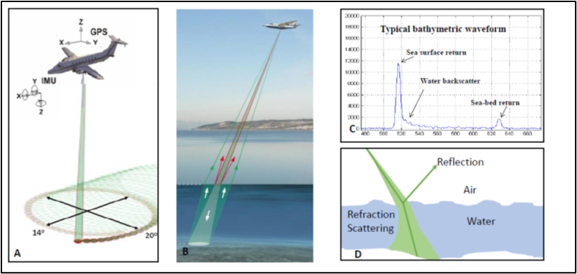
**Figure A1. Topo-bathymetric LiDAR (TBL) principles**

Text version - Figure A1. Topo-bathymetric LiDAR (TBL) principles

A - Typical elliptical scan pattern for TBL with navigation system GPS+IMU. Image taken and adapted from Leica Geosystems.

B- Most TBL system have a NIR and green laser.

C – Typical waveform captured from the green laser.

D – Interaction of the green laser light when travelling between air and water, refraction and scattering take place.

The main limiting factor affecting depth of penetration of TBL is water clarity. Thus, turbidity management is required for a successful survey. The main sources that can adversely affect the green laser from penetrating the water column come from suspended sediment, although algae blooms may also have negative impacts, as well as dissolved organic matter which can be common in some lakes and streams that originate in bogs. The water clarity fluctuations of a study site should be considered when planning a survey (See section ‘Guidelines for a Topo-Bathymetric LiDAR project). Moreover, the green laser of the TBL does not penetrate air bubbles (white caps, surf zone, etc.) as a result of the scattering. This has implications along coastlines with heavy surf that may need to be flown twice at different tide levels.

Flights operations, GNSS base stations set up and sensor calibration principles are similar to those of typical topographic LiDAR and thus are not presented here.

The processing of TBL data after a mission is like topographic data as the first step is to process the trajectory of the aircraft using a ground base station and the GNSS and inertial measurement unit in the sensor. During a TBL survey, the waveforms of the NIR and green laser are recorded and are related to the trajectory by GNSS time. Once related to the trajectory, the waveforms are then post processed into discrete points. During the processing of the green laser waveforms, the water surface is detected and modelled for the green laser pulse path to be refracted at the water surface and the range adjusted by the change of the speed of light in water. The typical recorded waveform from the green laser consists of a large amplitude return from the water surface followed by the volume backscatter of the laser pulse through the water column and then a peak representing reflection off the seabed or riverbed (Figure A1-C).

One distinct advantage of surveying hydrography with TBL when compared to echo sounding is that the speed of the light in water is only marginally affected by changes in salinity and temperature compared to how these properties effects on the speed of sound in water. This property makes TBL ideal for surveying in estuarine environments where fresh and saltwater mix in a sometimes-complex fashion.

Benefits of Topo-Bathymetric LiDAR for flood risk mapping

Most recent flood inundation maps were based on topographic LiDAR alone with no details of the bathymetry. Although the methods used to produce inundation maps from topographic LiDAR have been found to be reasonably accurate, these approaches do not calculate the speed of the flood water or the time and duration of inundation. In order to calculate these variables, one must utilize a hydrodynamic modelling software. One of the main parameters that controls the movement of water in a hydrodynamic model is the bathymetry. Other parameters also effect the movement of water including bed roughness, sometimes defined as Manning’s Roughness Coefficient, which effects the drag between the water and the bed. The results of TBL survey can provide information of topography and bed material (with LiDAR intensity) and have been used to construct benthic cover maps or habitat maps (Webster et al., 2016), which can be used to estimate bed roughness for hydrodynamic models.

Coastal flood risk is associated with elevated sea-levels associated with storm surges. In addition to elevated total water levels (tide+surge), waves and wave-runup can also cause additional flooding and erosion. In order to model the hydrodynamics of a storm surge event and possible wave set-up and run-up, a seamless DTM is required. In order to calculate wave set-up and wave run-up, near shore bathymetry is required (Olabarrieta and Warner, 2016). Nearshore bathymetry has been a challenge to map prior to TBL. Most techniques for mapping land elevation do not work in the coastal zone (e.g. photogrammetry, topographic LiDAR) and techniques to map the deep water such as boat-based echo sounding are dangerous and inefficient in shallow water. The ability of TBL to acquire seamless DTMs across the coastal zone into the near shore has enabled detailed hydrodynamic models to be constructed.

In the case of fluvial or inland flood risk mapping, many studies have used topographic LiDAR to map the exposed floodplain and estimate the river channel topography. Many fluvial models are based on 1-Dimensional hydrodynamic models, or 1-D models where cross-sections are extracted from the floodplain and river channel and used to calculate the momentum and mass of water moving through the section. Measuring riverbed cross-sections manually (e.g. Using GNSS, or boat-based echo sounding) is expensive and time consuming and in some cases dangerous to the operators. As a result, the channel topography is only measured in a few cross-sections and the remaining areas are estimated by interpolation or using an empirical relationship based on the exposed channel geomorphology. The discharge or flow (cubic meters per second) of a river is controlled by the channel bathymetry and gradient. The ability of TBL to acquire seamless elevation data of the floodplain and the river channel offers a great deal of potential to improve the accuracy of the cross-sections that are used in flood models.

Accuracy standards

The International Hydrographic Organization (IHO) specifies different Orders standard for bathymetric data in terms of total vertical or horizontal accuracy, at 95% confidence interval (IHO, 2008). The Order 1 standard applies for areas shallower than 100 m and Special Order is typically recommended for areas or applications requiring the highest accuracy of survey. The Total Vertical Uncertainty (TVU) varies with depth and is defined in the equation below, where ‘a’ represents the portion of uncertainty that does not vary with depth (e.g. airport position uncertainty from the trajectory processing), ‘b‘ represents the coefficient of the portion of the uncertainty that varies with depth ‘d’. All TBL system currently on the market can exceed the Order 1 requirements set out by IHO for depths less than 100 m (Saylam et al., 2018).

TVU = (a² + [b x d]²)^1/2

The following table describes the different IHO Orders and the horizontal and vertical accuracy expected.

**Table E1: IHO Orders and horizontal and vertical accuracies at 95% confidence interval (IHO, 2008).**
ORDER		Exclusive	Special	1a	1b	2	3 (Imprecise)
Examples of Typical Areas		Shallow water in Harbours, berthing areas, and associated critical channels with minimum under-keel clearances or engineering surveys.	Harbours, berthing areas, and associated critical channels with minimum under-keel clearances.	Areas shallower than 100 metres where under-keel clearance is less critical but features of concern to surface shipping may exist.	Areas shallower than 100 metres where under-keel clearance is not considered to be an issue for the type of surface shipping expected to transit the area.	Areas generally deeper than 100 metres where a general description of the sea floor is considered adequate.	All areas where the accuracies do not meet the requirements of the previous orders.
H	Horizontal Accuracy (95% Confidence Level)	1m	2m	5m + 5% of depth	5m + 5% of depth	20m + 10% of depth	>20m + 10% of depth
V	Depth Accuracy for Reduced Depths (95% Confidence Level) (1)	a = 0.15m b = 0.0075	a = 0.25m b = 0.0075	a = 0.5m b = 0.0013	a = 0.5m b = 0.0013	a = 1.0m b = 0.023	Same as order 2

In order to better appreciate how the TVU varies with depth for these different IHO orders, the TVU has been calculated at typical depths achieved by shallow water LiDAR sensors (15 m) and deep-water sensors (20 m and greater) (Table E).

**Table E2: Example of IHO orders and vertical accuracies (95% confidence) for depths 5, 10, 15, and 20 m.**
IHO Order	a	b	TVU (m) d=5m	TVU (m) d=10m	TVU (m) d=15m	TVU (m) d=20m
Exclusive Order	0.15	0.0075	0.15	0.17	0.19	0.21
Special Order	0.25	0.0075	0.25	0.26	0.27	0.29
Order 1a	0.5	0.013	0.50	0.52	0.54	0.56
Order 1b	0.5	0.013	0.50	0.52	0.54	0.56

Other bathymetric quality levels exist, such as the ones developed more recently through the “US’ National Coastal Mapping Strategy 1.0: Coastal Lidar Elevation for a 3-D Nation” (NSTC, 2016), but are not detailed in this appendix. Note that some of those quality levels are equivalent to the IHO Orders.

Acquisition Parameters Considerations

For TBL acquisitions for flood mapping and flood risks purposes, Table E3 provides summary of recommended acquisition parameters based on current scientific knowledge and available sensors.

**Table E3: Recommended LiDAR acquisition parameters for flood-related TBL acquisition.**
Parameters	Recommendation
Bathymetric point density	≥ 2 pts/m² (applicable for areas submerged at the time of survey).
Accuracy	Vertical and horizontal accuracies equivalent to IHO Special Order are recommended.
Swath overlap	20% minimum, but 50% is recommended
Flight altitude	400 m is recommended
Inland part	A minimum of 400 m inland horizontally, from the mean low water.
Depth of penetration of the LiDAR survey	Minimum 1.5 times the Secchi depth. The expected average penetration depth is 4 to 9 m in coastal areas, depending on water clarity. This value could be lower in some shallow rivers.
Maximum Scan angle	± 20 degrees is recommended (40 degrees field of view)
Time of acquisition	For areas affected by tides, acquisition should be made around low tide as much as possible (i.e. between two hours prior and two hours after low tide).

It is usually accepted that shallow water TBL are the sensors appropriate for flood risk studies and flood mapping. In cases where 2-3 Secchi depths need to be achieved at a lower point density for bathymetric coverage to support flood risk mapping, a combination of shallow and deep-water sensors may be suitable. Also, systems do exist that combine shallow and deep-water capabilities. Otherwise, the shallow water sensors provide the point density and penetration required to support most flood risk studies and can be supplemented with echo sounding data.
For TBL acquisitions related to hydrographic charting, the Canadian Hydrographic Service specifies that the spatial accuracy of the bathymetric portion of the TBL must meet the IHO Order 1b standards. They also specify deep-water TBL sensors capable of 2-3 Secchi depth of penetration in optimal conditions.

Guidelines for a Topo-Bathymetric LiDAR project

This section aims to provide some general guidance for a TBL project. The details and methods were inspired from the Canadian Hydrographic Services specifications, the NOAA specifications and the existing literature (e.g. Webster et al., 2016; Saylam et al., 2018).

A) Project planning and collection

During the mission planning phase and execution of the survey, the contractor must account for, demonstrate and implement strategies to mitigate the impact of the following parameters:

Topography of the survey area and surrounding area, such as mountainous terrain that could prevent or hinder flight operations.
Weather, including but not limited to water clarity and turbidity management. See the sub-section ‘Water clarity considerations’ below for more details.
Native phenomenon, such as kelp growth and algae blooms.
Maximum data acquisition around low tide. This is described as two hours prior and two hours after.
Include all bays, inlets, islands, peninsulas, inter tidal zones, flood plains, river deltas and land areas that are within the survey blocks.

The required point density is also important as it can influence how many flight lines are required and the level of overlap between survey lines. In general, if the desired point density can be achieved with a single flight line, then 20% overlap is sufficient to ensure there are no gaps during the collection process. A 50% overlap is recommended for flood-related TBL acquisitions to reduce data gaps and to ensure a more uniform distribution of points. It is understood that the requested density may not be met due to certain environmental conditions that cannot be controlled. Table E3 provides the recommended acquisition parameters for TBL acquisitions for flood-related applications.

The flight lines must be flown in alternate directions. They must also be planned to maximum expected depths, with the intention of collecting data to the point of extinction, not necessarily to the full extent of the survey blocks. Cross lines must be run across all planned LiDAR survey lines at angles ranging from 45 to 90 degrees more than the original survey line. Cross lines must be acquired and processed to the same accuracy and data quality standards as the main survey lines and may be included in the final product of the survey.

For shoreline mapping and modeling uses, it is particularly important to have good bathymetric data in the very shallow (0-4 m) areas. For this reason, the LiDAR systems, software, and processing procedures shall enable measurement of bathymetry in this very shallow region. The sensor used for this mapping shall have an operational measurement depth range equal to or greater than a 1.5 Secchi depth.

The time of acquisition must also be considered when conducting a TBL project. One challenge to TBL river surveys during full leaf-on conditions is the problem of overhanging vegetation obscuring the riverbed below. To overcome this, one could survey in the spring or fall during leaf-off conditions. The benefits of the leaf-off condition would have to be weighed against typical increased water levels and perhaps poorer water clarity conditions at that time of year.

Although not required, it is often desirable to have a field team on the water during the survey. The field team can collect Secchi depth readings to confirm the water clarity conditions (See the sub-section ‘Water clarity considerations’ for more details), and depending on the end application of the data, collect bottom samples and photographs to determine the benthic cover material. The field team would also collect check points both of hard surfaces on land and directly on the seabed to validate LiDAR data accuracy (see section ‘Data Validation’ below).

If coastal surveys are being conducted and any islands need to be surveyed, a twin-engine aircraft must be used in order to be able to safely make a landing if there is an engine failure. In addition to this safety requirement, most TBL surveys require a larger aircraft because of the increased power requirements for the green laser.

Water clarity considerations

For coastal and riverine TBL surveys, the weather proceeding a survey can greatly influence the conditions and probability of success. For example, in coastal areas, an onshore wind can cause waves which cause sediment to become suspended and thus high turbidity conditions where the particles in the water cause the light to scatter and not penetrate to the seabed. In the case of riverine environments, heavy rain can cause sediment and other organic materials to be transported into the river, thus degrading the water clarity. Turbidity management involves understanding the environmental conditions that cause high turbidity (e.g. wind and rain) and the length of time for the water to clear before it is suitable for a survey (Webster et al., 2016). A secondary factor affecting the depth of penetration of the green laser is the brightness of the seabed or riverbed. Darker objects have tendency to absorb the green light, while light objects, such as sand, reflect more of the green light and thus allow the signals to reflect back to the sensor at greater depths.

A Secchi disk is commonly divided into black and white quadrants in order to maximize contrast, and the depth at which the black and white disk disappears from view is called the "Secchi depth". Clear waters will have a larger Secchi depth than more turbid waters, and the size of the Secchi disk may need to be adjusted for different water clarity conditions (Philpot, 2019). TBL shallow water sensors typically have a depth rating of 1.5 times the Secchi depth, and deep water sensors have a rating of 2-3 times the Secchi depth.

Ideally when conducting TBL coastal surveys, there are multiple survey sites within the region that have different shoreline orientations such that not all sites will be turbid as a result of a regional wind event. It can be challenging to obtain Secchi depths leading up to a TBL survey and thus ensure the conditions are suitable. There are numerous terrestrial weather stations available on-line that can provide insights into the past and current wind and rain conditions; however it still can be challenging to predict the turbidity conditions, especially after a wind event when the water needs time to clear. This has led to the investigation of using real-time turbidity sensors that can be deployed in bays with different shoreline orientations or different geological and sedimentary conditions. These real-time turbidity buoys are equipped with a turbidity sensor and a communication package (e.g. cellular modem) that can transfer the readings to the internet to be checked remotely. This allows for a time-series of turbidity conditions to be measured and monitored prior to committing to a TBL flight.

Another approach to measure the water clarity is by using the Diffuse Attenuation Coefficient (Kd). The rate of change of the irradiance energy, E, is a function of the depth (Ed) and is a measure of water clarity that is similar in concept to the Secchi depth in that the rate of change will be faster in turbid waters than in clear waters. The rate of change of Ed, or logarithmic derivative of Ed, is the diffuse attenuation coefficient, Kd (Philpot, 2019).

k_{d} = - \frac{d ln E_{d} (z, λ)}{dz} = - \frac{1}{E_{d} (z, λ)} \frac{d E_{d} (z, λ)}{dz} (m^{-1})

Figure A2: Diffuse Attenuation Coefficient Kd, E(λ) radiance distribution over a hemisphere at a certain wavelength of energy (λ) at depth z (Philpot, 2019).

Kd values can change rapidly for a body of water, however the typical values of Kd range from 0.05 for clear water to 0.11 for turbid water for wavelengths used in TBL. For coastal areas, some medium resolution satellites, such as MODIS, can help estimate Kd or Secchi depth for certain wavelengths which can aid to determine if a TBL survey is feasible for an area or the best season to attempt a survey.

B) Data processing and management

Once the waveform data have been processed into discrete points (see section ‘Topo-bathymetric LiDAR general principles’ for more details), the classification is then typically performed. The points located in the bathymetric area must be classified according to the classes detailed in Table E4. We recommend that the points onshore be classified at least with the classes specified at section 5 of the current Guideline. Automatic and manual refinement of the classification are typically required using many of the standard tools that are used for topographic LiDAR processing. Most TBL system are equipped with a RGB or multispectral camera system that can be used to colorize the LiDAR point cloud and generate orthophotos. The coincident orthophotos can be very useful in assisting with the interpretation of some of the LiDAR returns.

**Table E4: Classification codes used for bathymetric features for the LAS 1.4 data (Excerpt from the topo-bathy LiDAR domain profile, July 2013)**
Classification Value	Meaning
40	Bathymetric point (e.g., seafloor or riverbed; also known as submerged topography)
41	Water surface (sea/river/lake surface from bathymetric or topographic-bathymetric lidar; distinct from Point Class 9, which is used in topographic- only lidar and only designates “water,” not “water surface”)
42	Derived water surface (synthetic water surface location used in computing refraction at water surface)
43	Submerged object, not otherwise specified (e.g., wreck, rock, submerged piling)
44	International Hydrographic Organization (IHO) S-57 object, not otherwise specified
45	No-bottom-found-at (bathymetric lidar point for which no detectable bottom return was received)

During data processing, all blunders and artifacts (boats, fisheries, weeds, etc.) must be assigned to class 1.

The delivered point cloud data and/or derived DEMs must be a seamless product (i.e. topographic and bathymetric LiDAR data joined), referenced to common horizontal and vertical coordinate reference systems. For flood risk studies, we recommend using the same coordinate reference systems than those recommended for topographic LiDAR data in the current Guideline (See section 6.3.3).

For hydrographic charting, it may be required that the bathymetric data be referenced to the Chart Datum. In some case, a separation model between the Chart Datum and ellipsoidal heights can be provided by the technical authority to perform vertical transformation. If no such file is provided, the vendor is encouraged to use the Canadian Continuous Vertical Datum for Canadian Waters (CVDCW) process and the applicable Hydrographic Vertical Separation Surfaces (HySEP or SEP) for the survey area. The HySEP/SEP provides the separation between Chart Datum and the GRS80 (NAD83(CSRS)) ellipsoid.

The delivered point cloud data must be classified and in a LAS 1.4 point cloud format. Intensity values must be required for each multiple discrete return. The values recorded in the LAS files shall be normalized to 16 bit, as described in the LAS Specification.

C) Data validation

Wherever possible, it is always recommended that independent check points of a high precision be collected to compare to both the topographic and bathymetric LiDAR points. The standard approach is to utilize RTK GNSS to collect check points in the floodplain and across the river channel. For more information on the validation methods for topographic LiDAR data, see section 6.4 from the current Guideline.

For the bathymetric portion of a TBL survey, horizontal and vertical accuracy requirements are defined using the IHO Orders as stated earlier (Section ‘Accuracy standard’). However, there are no set guidelines in terms of the number of check points required or their distribution for TBL surveys. As with all validation techniques, the check points used to validate the LiDAR points or surface models must be at least 3 times more accurate than the expected accuracy of the LiDAR.

It is recommended that for river TBL surveys, cross-sections be taken using survey grade GNSS positioning directly of the riverbed and where that is not possible using echo sounding techniques. These check points should be distributed to include examples of variable depths and conditions in the river.

In the case of coastal TBL surveys, direct measurements of the seabed elevation are possible using a GNSS antenna connected to an extendable pole, on the order of 4 m. This ensures direct measurements of the seabed for check points in shallow water. These check points must be taken near the time of the TBL survey, unless the seabed is comprised of exposed bedrock and is not expected to change over time. In deeper areas, echo sounding techniques can be used if the vertical accuracy of the data is suitable. As with topographic LiDAR, the expected vertical accuracy of TBL surveys will be influenced by the conditions of the seabed and will vary based on the presence, density and height of submerged aquatic vegetation (SAV). The TBL systems utilize green light which will not penetrate a dense canopy of SAVs, similar to topographic LiDAR and dense vegetation on land. Thus, when collecting check points on the seabed, it is also desirable to measure the presence and height of SAV.

D) Deliverables

Prior to the acquisition period, it is recommended that the contractor provide the technical authority with a project planning report containing details on team mobilization, GNSS and base stations data, water clarity monitoring approach, calibration reports and methods, as well as a detailed project schedule. The project planning could be subject to acceptance by the technical authority.

During the acquisition period, it is recommended that the contractor provide the technical authority with progress reports at regular intervals or following acquisition days.

Typical final deliverables for a TBL project may include the following items:

Seamless topo-bathymetric classified LiDAR files. In some cases, the combination of topographic and bathymetric point cloud may not be required. The raw point cloud could also be required in certain cases.
Seamless topo-bathymetric digital elevation models. Note that for some projects, the combination of topographic and bathymetric digital elevation models may not be required.
Final project report, including but not limited to data acquisition, data processing and quality assurance details, position techniques and ground control. This report should contain sufficient detail to demonstrate that the specifications have been met for each pulse data collected.
Final index showing coverage of the data with complete explanation of possible data gaps (e.g. depth extinction, water clarity, etc.).
Orthophotos taken simultaneously to the acquisition.
Metadata compliant with the ISO 19115:2003 standard.
Flight lines trajectory
Check points with horizontal and vertical accuracy estimates.
Depending on the variable uses of the data, flight line normalized LiDAR intensity model (NIR returns on land and green laser returns of the river-seabed).

References

Canadian Hydrographic Services (2013). Standards for Hydrographic Surveys. Edition 2.

International Hydrographic Organization (2008). IHO Standards for Hydrographic Surveys (Special Publication No. 44). Pp. 1-28. Monaco: International Hydrographic Bureau.

Klemas, V. (2011) Beach Profiling and LIDAR Bathymetry: An Overview with case studies. Journal of Coastal research 27(6), 1019-1028.

Legleiter, C. J., & Kyriakidis, P. C. (2008). Spatial prediction of river channel topography by kriging. Earth Surface Processes and Landforms, 33, 155–161.

McGuigan, K., Webster, T., Collins, K. (2015). A Flood Risk Assessment of the LaHave River Watershed, Canada using GIS Techniques and an Unstructured Grid Combined River- Coastal Hydrodynamic Model. Journal of Marine Science and Engineering, 3(3) ISSN 2077-1312; doi:10.3390/jmse3031093.

Olabarrieta, M. and Warner, J.C. (2016) Inwave: The Infragravity Wave Driver of Coast. COAWST Workshop. Woods Hole 2016.

National Oceanic and Atmospheric Administration Technical Memorandum NOS CS 32 (2013). A procedure for developing an acceptance test for airborne bathymetric lidar data application to NOAA charts in shallow waters.

National Science Technology Council (2016). National Coastal Mapping Strategy 1.0: Coastal Lidar Elevation for a 3-D Nation (PDF, 4.6 mb).

Philpot, William (2019). Airborne Laser Hydrography II.

Saylam, K., Hupp, J.R., Averett, A.R., Gutelius, W.F., and Gelhar, B.W. (2018). Airborne lidar bathymetry: assessing quality assurance and quality control methods with Leica Chiroptera examples. International Journal of Remote Sensing. Vo. 30 No. 8; doi: 10.1080/01431161.2018.1430916 pp. 2518-2542.

Webster, T., McGuigan, K., Crowell, N., Collins, K. and MacDonald, C. (2016). Optimization of data collection and refinement of post-processing techniques for Maritime Canada’s first shallow water topographic-bathymetric lidar survey. Journal of Coastal Research. Special issue on Advances in Topo-Bathymetric lidar. Vol 76: doi:10.2112/SI76-004, pp. 31-43.

Appendix 6 – Contract

The guideline reflects specifications for collecting airborne LiDAR data and contracts identify specific requirements, enhancements or changes to the guidelines. Key contract items included are listed below.

Definitions

Include a reference list of terms used in contract with definition.

Vendor Information

Provide information about the vendor including legal name, operational centre, and contact information.

Scope

Project specific requirements would be specified in this section. They would include data requests such waveform data, increase quality assurance where the vendor requires more sampling, and higher pulse density. A schedule and detailed deliverables would be clearly listed.

Some specific project scope contract items to be consider by the contracting authority are as follows:

DCAOI
Pulse density required
Review of methodology
Deviation from instrumentation
Vertical and horizontal accuracy
Request for intermediate or waveform pulse data
Data collection period
Check points consideration including the number and who will conduct this
Data ownership and usage
Contingency plan
Time period for data validation and verification on project deliverables
Raw data requirements
Additional post classification fields
Any derivative products i.e. DEM, contours, hydro-flattening
Tile sizes, file format and naming convention
Waivers or adjustment for high relief areas, snow and vegetation conditions
Accepting compress LAZ files
Use of Virtual Reference Systems
Number of classification check
Conditions for rejecting the data e.g. data voids or density

Insurance

Insurance coverage for aircraft and automobile is required. This would include Commercial General Liability and Errors and Omission. Specific liability amount would be identified. The contract authority would be identified as rider on the insurance.

Confirm Insurance coverage and requested certificate
Confirm Workplace Safety Insurance Coverage

Safety

Workplace safety plan would be provided to ensure the safety in data collection particularly in remote locations. This would include identification of hazards, risk assessment, mitigation plan and required safety gears. Safety consideration must follow all federal and provincial government regulations. Examples include: vehicle roadside safety, hours of data collection and wildlife hazards.

Request vendor health and safety plan

Termination Clause

Identify the conditions where a vendor fails to perform duties or breaches contract. A termination clause would be included in the contract identifying conditions for termination.

Dispute Resolution

Should a dispute in the terms and condition of the requirements and contract occur, this section would cover a detailed process for dispute resolution including notification by vendor or contracting authority, mediation and actions that can be taken.

Wavier

Any exceptions or adjustments by the contracting authority with the terms and conditions of the contract and data collection requirements are to be put into writing to be valid.

Deliverable Review Period

The vendor will provide as part of its deliverable early in the project a plan with methodology for meeting the guideline with respect to data collection, processing and deliverables. A time period is required for the review of the processing and to inspect and accept the deliverables. Terms would be included and a completion certificate for accepted work would be submitted by the vendor.

Payment Terms

Financial payments for the project would consider the upfront costs for airborne operations and the deliverables. Milestone payment and percentage of payment would be structured in the contract. Any withholding would be identified.

Subsuppliers and Subcontractors

Any additional changes of subsuppliers and subcontractors would require written consent by the contract authority for any changes. Workplace safety and all insurance requirements must be enforced with subsuppliers and subcontractors.

Force Majeure

A description outlining a breach of contract due to events such as war, riot, fire, sabotage, national security and other events or circumstances which are not reasonably foreseen and which have not been caused by an act, omission or negligence and is beyond the control of the vendor or contracting authority is included and what conditions and notification would transpire.

Entire Agreement

The contract is to contain all conditions, requirements and specifications. No other terms, agreements or conditions shall be binding.

Performance of Services

A clause indicating time of essence and agreement to perform the required task with the agreed schedule. The contracting authority may terminate the contract upon a default of agreed upon conditions.

Permits

A clause identifying any permits for flying, ground access or other requirements to provide the service and products is required by the Vendor at its own cost.

Compliance with Law

A clause is placed to bind the vendor and any subcontractors, agents, contractors to comply to all applicable laws and regulations at all levels of government. Vendor also indemnify the contract authority from any negligence occurring on behalf of the Vendor, its agents, contractors and subcontractors.

Expediting

A clause may be placed to expedite work and delivery of product should it become apparent that the schedule will not be met.

Warranty

Any warranty with the deliverables shall be provided. Warranty will cover compliance with specifications, quantity and quality. The warranty shall have a period of time and period in which non-conformity would be rectified. The warranty clause may contain any potential liability arising from defected product.

Governing Laws

The laws in which the contract applies can be provincial, federal and/or international laws.

Indemnity

The contract would contain clauses with respect to indemnification arising from not performing the service or delivering the product or negligence in the operation of collecting the data or any other breach of contract.

Confidentiality

Information provided to the vendor by the contracting authority identified as confidential information shall protect the information from unauthorized use, disclosure and duplication of content.

Successors and Assignments

A clause would restrict a vendor from transferring the contract to another party without the consent of the contracting authority. The clause would stipulate the contracting authority’s rights to accept or deny the request.

Data Ownership

This designates the assignment of rights and ownership of the data to the contracting authority. The data ownership model determined between the contracting authority and vendor is on a project by project basis.

Page details

Date modified:: 2024-06-18