
Federal Hydrologic and Hydraulic Procedures for Flood Hazard Delineation
Version 2.0, 2023
Natural Resources Canada General Information Product 113e,
Natural Resources Canada, Environment and Climate Change Canada Public Safety Canada
© His Majesty the King in Right of Canada, as represented by the Minister of Natural Resources, 2023
For information regarding reproduction rights, contact Natural Resources Canada at copyright-droitdauteur@nrcan-rncan.gc.ca.
Preface to the second edition
The Federal Flood Mapping Guidelines Series was established in 2015 to summarize current approaches to flood mapping in Canada. The series is intended to facilitate the development and application of best practices and increase the sharing and use of flood hazard information. The first edition of this document was published in 2019.
This second edition of the Hydrologic and Hydraulic Procedures for Flood Hazard Delineation expands on key topics and aims to provide improved guidance on climate change, uncertainty, and lakeshore flooding. Several approaches for incorporating climate change effects in flood delineation studies are being explored at municipal, provincial/territorial, and federal levels of government. It is anticipated that these guidelines will continue to be updated on a regular basis to reflect current best practices for incorporating climate change into flood hazard delineation studies in Canada. The section on uncertainty was expanded in this edition to describe approaches for handling uncertainty including periodic review and adaptive management. The section on coastal flooding was also rewritten to focus exclusively on lakes, as a new guideline document on marine coastal flooding will be published. The section on lakeshore flooding provides guidance on flooding due to high lake levels, storm surge, and wave effects.
The document was also reorganized to meet the needs of two target audiences. The first three sections provide an overview of the general practices for undertaking flood hazard delineation studies and were written for local governments procuring technical studies and individuals or organizations involved in flood management. The six sections that follow provide a summary of accepted technical practices for defining extreme flows and water levels and are intended for practitioners. Section 10.0 and Appendix A are new to this edition and describe suggested reporting requirements. They are intended for organizations who undertake or who procure flood hazard delineation studies. A table of revisions is included after the Table of Contents to assist readers familiar with the first edition of the guidelines.
Several new topics were considered for this edition of the guidelines but were excluded due to time constraints. Future versions of the guidelines may include guidance on urban stormwater management; geohazards, such as debris flows and alluvial fans; and geomorphic changes.
Table of contents
- Preface to the second edition
- 1.0 introduction and purpose
- 2.0 General practices
- 3.0 Data requirements
- 4.0 Incorporation of climate change
- 5.0 Procedures to assess design flood events
- 6.0 Hydraulic analysis
- 7.0 ice effects
- 8.0 Lakeshore flooding
- 8.1 Physical Processes
- 8.2 Data Requirements
- 8.3 Meteorological Data Analysis
- 8.4 Static Lake Level Analysis
- 8.5 Storm Surge Analysis
- 8.6 Wave Analysis
- 8.7 Wave Generation
- 8.8 Nearshore Wave Transformation
- 8.9 Wave Runup and Overtopping Analyses
- 8.10 Mapping Lakeshore Flood Hazards
- 8.11 Climate Change Considerations
- 8.12 Lakeshore Flood Frequency Analysis
- 8.13 Reporting Requirements
- 8.14 Summary of Practices for Lakeshore Flooding
- 9.0 Uncertainty in flood hazard assessment
- 10.0 Requirements for report format
- 11.0 Conclusion
- 12.0 References
- 13.0 Bibliography
- Appendix A: requirements for technical reports
List of tables
- Table 2.1 - General practices for flood hazard delineation
- Table 2.2 - Application of 1-D and 2-D hydraulic models
- Table 4.1 - Practices to incorporate climate change into flood hazard studies
- Table 5.1 - Hydrologic practices
- Table 5.2 - Hydrologic outcome or design flood event by jurisdiction at the time of writing
- Table 5.3 - Basis for classifying hydrologic simulation models (adapted from Associate Committee on Hydrology, 1989)
- Table 6.1 - Fluvial hydraulic practices
- Table 6.2 - Application of various hydraulic models
- Table 7.1 - Ice-jam flood assessment practices
- Table 8.1 - Lakeshore flood hazard analysis and mapping procedures
List of figures
- Figure 0.1 - Flood Mapping Framework
- Figure 2.1 - General practices for flood hazard delineation
- Figure 2.2 - Hydrology and system hydraulics procedures
- Figure 2.3 - Focus of hydrologic requirements in flood hazard delineation
- Figure 2.4 - Hydrologic design methodologies
- Figure 2.5 - Length of record constraints on hydrologic procedures
- Figure 2.6 - Hydrologic modelling framework
- Figure 2.7 - Hydraulic requirements in flood hazard delineation
- Figure 2.8 - Typical processes leading to ice jams
- Figure 2.9 - Elements of overall uncertainty
- Figure 3.1 - Data requirements for flood hazard delineation
- Figure 4.1 - Climate change application
- Figure 5.1 - Hydrologic procedures
- Figure 5.2 - Procedure for preparing flows for analysis
- Figure 5.3 - Naturalization of regulated flows
- Figure 5.4 - Procedure for flood frequency analyses
- Figure 5.5 - Hydrologic modelling approaches
- Figure 5.6 - Deterministic hydrologic models
- Figure 5.7 - Requirements for hydrologic modelling for flood frequency analyses
- Figure 5.8 - Steps in model application
- Figure 6.1 - Hydraulic modelling procedure
- Figure 6.2 - Calibration and validation of a hydraulic model
- Figure 7.1 - Ice-jam procedure
- Figure 8.1 - Static water level anomalies on Great Slave Lake at Yellowknife (1939–2018)
- Figure 8.2 - Lake Erie long-term water level variations
- Figure 8.3 - Estimation of storm surge and static water levels from long-term water level gauge records
- Figure 8.4 - Cox-Machemehl method for estimating wave overtopping-induced hazards
- Figure 8.5 - Definition of lakeshore flood hazards for wave runup and overtopping
- Figure 9.1 - Uncertainty of hydrologic and hydraulic modelling
| Section | Update |
|---|---|
| Context | expanded description of flood sources |
| Federal Flood Mapping Framework | updated figure and description |
| Federal Flood Mapping Guidelines Series | updated with latest publications in guidelines series |
| List of Abbreviations And Acronyms | updated |
| 1.0 Introduction And Purpose | moved sections on: Note on Terminology, Standard of Care, Regulatory Regimes, and Risk-based Decision Making to the introduction; added section on Background and Scope |
| 1.4 Note on Terminology | updated to comply with other documents in series |
| 1.5 Standard Of Care | clarified qualifications of practitioners |
| 1.6 Regulatory Regimes In Canada | corrected definition of Ontario's CAs |
| 2.0 General Practices | reorganized section and expanded descriptions for a non- technical target audience |
| 2.1 Scope Of Work Requirements | defined requirements of scope of work for a flood hazard delineation study |
| 2.2 Design Flood Assessment | added high-level overview of processes with flow charts |
| 3.0 Data Requirements | created new section to consolidate data requirements subsections in previous version |
| 4.0 Incorporation Of Climate Change | moved section from end of document; created new figures and explanations |
| 4.1 Climate Change Information Data | revised and reorganized section |
| 4.4 Summary Of Strategies For Consideration Of Climate Change | created new section |
| 5.0 Procedures To Assess Design Flood Events | reorganized and updated section |
| 5.1 Definition Of Hydrologic Outcome | created new section |
| 5.2 Data Requirements | created new table, figures, and explanations on flow analyses |
| 5.3 Selection Of Analytical Approach | created new figure and explanation |
| 5.4 Flood Frequency Analysis Approach | revised and reorganized section; new figure and explanation |
| 5.5 Hydrologic Modelling | created new figures and explanations |
| 5.8 Summary Of Hydrologic Procedures | created new section |
| 6.0 Hydraulic Analysis | reorganized and updated section |
| 6.1 Model Selection | created new tables, updated references |
| 6.2.1 Geospatial Data | created subsection on topography and bathymetry |
| 6.2.8 Stage-Discharge Relationships | clarified application of rating curves |
| 6.3 Sensitivity Analysis, Model Calibration, And Model Validation | created new section |
| 6.5 Summary Of Hydraulic Procedures | created new section |
| 7.0 Ice Effects | added flow chart and table |
| 7.6 Hydraulic Analysis To Account For Ice Effects | created new section |
| 8.0 Lakeshore Flooding | updated section for lakeshore flooding; removed information pertaining only to marine coasts |
| 9.0 Uncertainty In Flood Hazard Assessment | updated section |
| 10.0 Requirements For Report Format | created new section for reporting requirements |
| 11.0 Conclusion | updated to include purpose and limitations of scope |
| 12.0 References | updated |
List of abbreviations and acronyms
- 1-D
- One Dimensional
- 2-D
- Two Dimensional
- 3-D
- Three Dimensional
- AAFC
- Agriculture and Agri-Food Canada
- AEP
- Annual Exceedance Probability
- AES
- Canadian Atmospheric Environment Service
- AM
- Annual Maximum
- ANFIS
- Adaptive Neuro-Fuzzy Inference Systems
- ANN
- Artificial Neural Networks
- CaPA
- Canadian Precipitation Analysis
- CCCS
- Canadian Centre for Climate Services
- CFD
- Computational Fluid Dynamics
- CFSR
- NOAA’s Climate Forecast System Reanalysis
- CHS
- Canadian Hydrographic Service
- CIRNAC
- Crown-Indigenous Relations and Northern Affairs Canada
- cm
- Centimetre
- CMIP
- Coupled Model Inter-Comparison Project
- CORDEX
- Coordinated Regional Climate Downscaling Experiment
- CSA
- Canadian Space Agency
- DFO
- Fisheries and Oceans Canada
- DHI
- Danish Hydraulics Institute
- DTM
- Digital Terrain Model
- ECCC
- Environment and Climate Change Canada
- EGBC
- Engineers and Geoscientists British Columbia
- ESM
- Earth System Model
- FEMA
- Federal Emergency Management Agency (USA)
- FDRP
- Flood Damage Reduction Program
- FFA
- Flood Frequency Analysis
- FHIMP
- Flood Hazard Identification and Mapping Program
- GHG
- Greenhouse Gas
- GIS
- Geographic Information System
- GCM
- Global Climate Model or General Circulation Model (used interchangeably)
- GOC
- Government Operations Centre (Canada)
- GPS
- Global Positioning System
- GSDE
- Global Soil Datasets for Earth systems modelling
- IDF
- Intensity-Duration-Frequency
- INRS-ETE
- Institute national de la recherche scientifique – Eau Terre Environnement
- IPCC
- Intergovernmental Panel on Climate Change
- ISC
- Indigenous Services Canada
- JPA
- Joint Probability Analysis
- km
- Kilometre
- km2
- Square kilometre
- LiDAR
- Light Detection and Ranging
- m
- Metre
- m/s
- Metres per second
- m3/s
- Cubic metres per second
- mPING
- Meteorological Phenomena Identification Near the Ground
- MSM
- Multi-Objective Simulation Method
- NDMP
- National Disaster Mitigation Program
- NGO
- Non-Governmental Organization
- NHN
- National Hydro Network
- NOAA
- National Oceanic and Atmospheric Administration (USA)
- NRC
- National Research Council
- NRCan
- Natural Resources Canada
- NSERC
- National Sciences and Engineering Research Council
- PCIC
- Pacific Climate Impacts Consortium
- Probability Density Function
- POT
- Peaks Over Threshold
- PSC
- Public Safety Canada
- QA/QC
- Quality Assurance/Quality Control
- QD
- Mean Daily Peak Flow
- QP
- Instantaneous Peak Flow
- RCM
- Regional Climate Model
- RCP
- Representative Concentration Pathway
- RDRS
- Regional Deterministic Reforecast System
- RFFA
- Regional Flood Frequency Analysis
- RFP
- Request for Proposal
- RSL
- Relative Sea Level
- SCS
- Soil Conservation Service (US)
- SSP
- Shared Socioeconomic Pathways
- UAV
- Unmanned Aerial Vehicle
- USACE
- United States Army Corps of Engineers
- USACE HEC
- USACE Hydrologic Engineering Center
- USGS
- United States Geological Survey
- USIM
- Uncertainty Sensitivity Index Method
- WMO
- World Meteorological Organization
- WSC
- Water Survey of Canada
1.0 Introduction and purpose
This document, Federal Hydrologic and Hydraulic Procedures for Flood Hazard Delineation Version 2.0, is written for municipal, provincial, and territorial agencies and Indigenous communities working to produce flood hazard maps. It provides an overview of the technical procedures for flood delineation studies and is intended to assist those agencies in contracting the work or conducting the work itself. As described in Chapter 3 of the Federal Flood Mapping Framework Version 2.0:
“The documents contained in the Federal Flood Mapping Guidelines Series are to be used as a resource for flood mapping projects and activities undertaken across Canada. These guidelines aim to provide advice to provinces and territories, whose responsibility it is to provide technical guidance to implementing bodies, as well as individuals and organizations in Canada that need to understand and manage flood risks and their consequences to communities. They may include emergency management practitioners, flood risk managers, land-use and water resources planners, town planners, hydrologists, hydraulic engineers, geoscientists, geologists, infrastructure providers, water managers, and policy and decision makers, both within and outside of government.”
Flood management in Canada is regulated at the provincial, territorial, and municipal levels of government, and technical methods vary among jurisdictions. Federal programs exist to support Indigenous communities undertaking flood mapping studies. At the time of writing, First Nation communities south of the 60th parallel are eligible for funding of flood mapping studies under Crown-Indigenous Relations and Northern Affairs Canada (CIRNAC)’s First Nation Adapt Program. Indigenous Services Canada (ISC)’s Emergency Management Assistance Program provides funding to First Nation communities on reserve land to support hazard-risk assessments that can include flood mapping. Additionally, CIRNAC’s Climate Change Preparedness in the North Program provides funding to Indigenous and northern communities north of the 60th parallel to support hazard-risk assessments and maps that can include flood mapping.
This document provides a summary of the current technical practices used by practitioners of flood delineation in Canada. Officials at the provincial, territorial, and municipal levels of government and Indigenous communities may use this document to assist in scoping the work and ensuring that practitioners follow recognized and accepted practices.
These practices are not intended to supersede other federal, provincial, territorial, or local legislation, regulations, bylaws, policies, program standards, or technical guidance. The information and perspectives in this federal document do not necessarily reflect those of any individual provinces and territories or Indigenous communities. The methods outlined in this document are reflective of current technical practices in use in Canada and elsewhere.
1.1 Background and history
The first national guidelines for flood hazard delineation were published in 1976 as part of the Flood Damage Reduction Program (ECCC, 1976). These guidelines described the technical procedures and criteria to be followed for projects funded under the program. Thereafter, several provinces developed their own technical guidelines, often providing more extensive and prescriptive guidance and addressing local technical issues.
The creation of the National Disaster Mitigation Program (NDMP) in 2015 brought renewed funding for flood mapping and the development of the Federal Flood Mapping Guidelines Series. In 2019, an updated national guideline that summarized the hydrologic and hydraulic procedures for flood hazard delineation studies came out under this federal series. Members of federal, provincial, territorial, and municipal agencies, researchers, and practitioners reviewed the first version of the document.
This document (version 2) attempts to improve on the presentation of the concepts in version 1 by using explanatory flow charts, and reorganizing some of the content. The revision table after the table of contents details the changes made between the two versions.
Valuable input on the second version was received from the contributors to the first version and subject matter experts at ECCC. Members of provincial and territorial government agencies contributed their perspectives, and it is hoped that this document meets their needs for carrying out flood delineation studies.
1.2 Scope
The purpose of this document is to provide technical guidance on hydraulic and hydrologic procedures for preparing flood hazard maps in a Canadian jurisdiction. The specific objectives of this document are to:
- Describe the process that should be expected from practitioners providing technical flood hazard delineation services, including quality management and technical review.
- Describe different types of flooding that occur in Canada, including but not limited to fluvial (riverine), coastal (lakeshores), and ice-affected, alone and in combination. Urban stormwater management, debris flows, alluvial fans, geomorphic changes, and catastrophic events, such as a dam/dike/levee failures are not addressed in this document.
- Provide guidance for practitioners to conduct hydrologic and hydraulic analyses as part of the flood mapping process.
- Provide guidance on approaches and considerations for incorporating climate change into flood hazard studies.
As mentioned above, the Federal Flood Mapping Guidelines Series is a set of eleven documents published by the Government of Canada to provide technical guidance to individuals and organizations involved in flood mapping activities in Canada. As of the completion of this report, seven of the eleven documents have been published; the remaining documents are in progress and are expected to be released in 2023.
The scope of this document is focused on hydrologic and hydraulic analyses; guidance on mapping and geospatial data dissemination is provided in the Federal Flood Mapping Guidelines Series document titled Federal Geomatics Guidelines for Flood Mapping. Examples of projects incorporating climate change considerations in flood mapping are provided in a separate document in the Federal Flood Mapping Guidelines Series titled Case Studies on Climate Change in Floodplain Mapping.
1.3 Context for Risk-Based Decision Making
The federal government has acknowledged, through previous and current flood mapping programs, and as a signatory to the Sendai Framework on Disaster Risk Reduction, that floods and other natural hazards should be managed based on the principles of risk. A hazard must be considered along with the negative consequences of the events occurring. Understanding hazard frequency and severity (and variations to the frequency and severity over time due to climate and land use changes) is a cornerstone of this approach and is the focus of this document. A companion document in the Federal Flood Mapping Guidelines Series titled Federal Guidelines for Flood Risk Assessment will provide guidance on the other components of risk (exposure, vulnerability, and resilience) when it is released.
1.4 Note on Terminology
All Federal Flood Mapping Guidelines Series documents will apply the following definitions, based on the Emergency Management Framework for Canada (Ministers Responsible for Emergency Management, 2017) and NDMP (NDMP, 2021) literature. It is recognized that provinces and territories may define these terms differently, and these definitions are not intended to be prescriptive outside the context of the Federal Flood Mapping Guidelines Series documents.
Flooding: The temporary inundation by water of normally dry land.
Flood Mapping: The delineation of a flood on a base map. This typically takes the form of flood lines on a map that show the area that will be covered by water, or the elevation that water would reach during a specified flood event. The data shown on the maps, may also include flow velocities, depth, other risk parameters, and vulnerabilities.
Hazard: A potentially damaging physical event, phenomenon, or human activity that may cause the loss of life or injury, property damage, social and economic disruption, or environmental degradation.
Risk: The consequence of a specific hazard, expressed in terms of likelihood, and based on considerations of vulnerability and exposure.
Flood maps are used for several different purposes, including identifying hazards and risks, land-use planning, emergency planning and response, and public awareness and communication. Under the broad definition of “flood map”, different types of geospatial, hydraulic, and hydrologic information can be presented to meet specific assessment requirements. The main types of flood maps can be found here.
For the purposes of this document, the following definitions also apply:
Annual Exceedance Probability (AEP): The probability, expressed as a percentage, of a given flood flow or water level occurring or being exceeded in any given year. Flood events are usually expressed in terms of an annual exceedance probability (AEP) or return period. For example, a 1% AEP flood event, and a 100-year flood event, are equivalent. However, the concept of return periods is sometimes misinterpreted by non- technical audiences as a period of time between events (e.g., 100 years until the next 100-year flood) rather than an annual probability.
Design or Regulatory Flood: A specific flood magnitude that is used for delineating flood hazard areas.
Digital Terrain Model (DTM): A land surface, free of buildings and vegetation, represented in digital form by an elevation grid or lists of three-dimensional coordinates.
Flood Hazard Area: The area inundated by flood waters for the design or regulatory event, as determined by hydrologic and hydraulic procedures.
Flood Hazard Delineation: The hydrologic and hydraulic procedures necessary to define the extent, depths, and velocities of the design or regulatory flood for mapping on the study area.
Floodplain: Areas adjacent to the river channel, lake shoreline, or coastline that are subject to flooding.
In some jurisdictions, the floodplain is divided into the floodway and the flood fringe. In jurisdictions where this division exists, the terms are often defined as follows:
Floodway: The river channel and adjacent areas where water depths and velocities are greatest and most hazardous.
Flood Fringe Areas: The remaining areas of the floodplain that are outside of the floodway.
Hydrometric: Relating to the monitoring and recording of water levels, velocities, and flows.
Hydrotechnical: Relating to the technical aspects of water resources (e.g., flows, levels, extents, velocities).
Riverine/Fluvial Flooding: The temporary inundation of normally dry land by water that escapes the river channel and flows onto the adjacent floodplain and which may be caused by rainfall, snowmelt, stream blockages including ice jams, failure of engineering works, or other factors.
Stream: A general term used to describe watercourses including streams and rivers. Throughout the document, “stream” and “river” are used interchangeably.
Streamflow: The volume of water passing by a specific point in a stream at a defined interval. Often referred to as discharge (e.g., in cubic metres per second—m3/s). Throughout the document “streamflow”, “flow”, and “discharge” are used interchangeably.
Study Stream: The stream that is the focus of the flood study.
Study Site: The location of the flood hazard delineation.
Watershed: The drainage basin, including tributary basins, above the study site.
1.5 Standard of Care
Flood hazard maps are critical tools for disaster mitigation planning and emergency management, including protection of life and property. In addition, flood hazard maps are essential for land-use planning, zoning, insurance, and communication of flood-related risks to the public. The flood hazard delineation process, including hydrologic and hydraulic analyses, must be conducted in accordance with safety and standard of care requirements, such as those described by provincial and territorial geoscience and engineering regulatory bodies.
Engineers and geoscientists are required to provide the standard of care described by professional engineering and geoscientist associations in the province or territory where they practise. Engineers and geoscientists practising in a Canadian jurisdiction must be registered members of the professional association for that jurisdiction, and must comply with the requirements of the acts, regulations, bylaws, and the required standards of care. Provincial or territorial legislation regulates the licencing functions of these associations. The practices in this document (Federal Hydrologic and Hydraulic Procedures for Flood Hazard Delineation) submit to all acts, regulations, bylaws, or any other requirements of provincial or territorial professional engineering and geoscience associations.
Specific requirements for the professional practice of engineers and geoscientists preparing flood maps in Canadian provinces and territories include, but are not limited to:
- Holding paramount the safety, health, and welfare of the public and protection of the environment.
- Complying with acts, regulations, bylaws, and standards of care (e.g., as outlined in guideline documents published by the relevant provincial or territorial professional engineering and geoscience association).
- Possessing the appropriate level of training and experience to carry out flood mapping in that geographic area.
- Engaging interested parties and specialists as needed.
- Establishing a mechanism for internal checking and review, which may include independent peer review.
For the purposes of this document, a “qualified professional” signifies someone who possesses the specialized knowledge and experience required to conduct hydrologic and hydraulic analyses to support flood mapping, licensed under the Canadian provincial or territorial engineering regulator for the study site. This document provides an overview of accepted methodologies for undertaking flood hazard delineation studies; a qualified professional may use other procedures providing they follow accepted engineering practice. In this document, “practitioners” can include qualified professionals or other people working for them, where the qualified professional would verify the work and do the final sign-off.
1.6 Regulatory Regimes in Canada
In Canada, flood management is primarily the responsibility of the provinces and territories, and may be delegated to municipalities and conservation or watershed authorities through legislation. Therefore, some flood management activities, including mapping, planning, preparation, response, and recovery, are executed at a delegated level (e.g., Ontario Conservation Authorities, Manitoba Watershed Districts) rather than provincial, territorial, or federal levels. However, provincial and territorial legislation generally includes provisions requiring municipalities or other responsible organizations to undertake flood mitigation and emergency response actions deemed necessary in the public interest. The authority to set the design flood hazard measure, whether a single probability, multiple probabilities, or extreme design event, is at the provincial/territorial level.
Federal programs exist to support Indigenous communities undertaking flood mapping studies. At the time of writing, First Nation communities south of the 60th parallel are eligible for funding of flood mapping studies under Crown-Indigenous Relations and Northern Affairs Canada (CIRNAC)’s First Nation Adapt Program. Indigenous Services Canada (ISC)’s Emergency Management Assistance Program provides funding to First Nation communities on reserve land to support hazard-risk assessments that can include flood mapping. Additionally, CIRNAC’s Climate Change Preparedness in the North Program provides funding to Indigenous and northern communities north of the 60th parallel to support hazard-risk assessments and maps that can include flood mapping.
The federal government has three general areas of responsibility relating to flooding in Canada, each involving coordination with provinces and, in some cases, municipalities:
- Monitoring of and response to Canadian flood situations through the Government Operations Centre (GOC), which coordinates federal government responses to flood events of national significance.
- Provision of disaster assistance, including Disaster Financial Assistance Arrangements, for the provinces and territories to address flood-related financial losses.
- Implementation of federal flood mapping programs (e.g., Flood Hazard Identification and Mapping Program [FHIMP]), including support for flood mapping activities used to mitigate flood risks and costs and to reduce or negate the effects of flood events in Canada.
1.7 Document Outline
The following sections in this document are organized into two themes. Sections 2.0 and 3.0 are intended for an audience without a technical background and describe the general hydrologic and hydraulic procedures and data requirements for undertaking a flood hazard delineation study. They include the following key items:
- Overview of hydrologic and hydraulic procedures.
- Scope of Work requirements for inclusion in a Request for Proposal (RFP).
- Overview of flood frequency analysis and hydrologic modelling.
- Overview of approaches and strategies to assess the effects of climate change on specific flood mechanisms.
- Overview of hydraulic modelling.
- Overview of ice-related flooding and ice-jam processes.
- Overview of lakeshore flooding.
- Overview of uncertainty in flood hazard delineation results.
- Summary of suggested reporting requirements.
- Data requirements.
Sections 4.0 to 10.0 are more technical and are written for practitioners who would be undertaking and/or reviewing the work. They include the following key items:
- Hydrologic procedures for flow adjustments, flood frequency analyses, and hydrologic modelling.
- Potential flood mechanism-specific techniques to assess the effects of climate change.
- Hydraulic modelling procedures, including model selection, development, and validation.
- Ice-related flood modelling including ice-affected or ice-jam flood frequency and hydraulic analyses.
- Lake flooding including procedures for static water level analyses, storm surge modelling and analyses, wave modelling, and wave runup and overtopping analyses.
- Techniques for quantifying uncertainty in the results and suggestions for addressing uncertainty.
- Detailed reporting requirements.
2.0 General practices
This section provides a general overview of the technical practices for flood hazard delineation. Section 2.1 describes scope of work considerations for flood hazard delineation projects. Section 2.2 outlines hydrologic procedures to assess design flows and/or water levels. Section 2.3 introduces approaches and considerations to assess climate change effects. Section 2.4 describes the application of hydraulic models that can be used to determine the depths, extents, and, in some cases the velocities, of the design flood at the study site. Section 2.5 describes ice-related flooding, and Section 2.6 lakeshore flooding. Section 2.7 describes techniques to assess and communicate uncertainty of the flood hazard delineation results. Finally, Section 2.8 outlines recommended reporting details to ensure that important details of the analyses are documented.
A summary of general practices for a flood hazard delineation study is included in Table 2.1, which occurs in three paths. Figure 2.1 shows a graphical representation of the framework and outlines the general practices.
| General Practices | |
| Step 1 | Define regulatory requirements based on legislation and the accuracy needed based on local land-use and zoning provisions for the study stream and surrounding area. |
|---|---|
| Step 2 | Determine study limits: providing the context of the geographic extent of the study body of water, impacts to be considered (fluvial, pluvial, ice, coastal, groundwater, debris flows, etc.). Determine sources of geospatial, hydrometric, meteorological, and historical systematic and non-systematic data. If necessary, include ice and/or coastal data sources specific to the impacts on flooding of the study location. Historical reports of flooding and its causes, as well as previous studies, are invaluable. |
| Path A | Determine the base mapping available:
Provide topographic mapping to qualified professionals for hydrotechnical analyses. |
| Path B-1 | Conduct the required hydrotechnical analyses using the skills and experience of a qualified professional, as defined in this document. |
| B-2 | Establish and use a mechanism for internal and/or external checking and review for each project. |
| B-3a | Perform the basic hydrologic analyses needed to determine the preliminary design flow or water levels. |
| B-3b | Incorporate future non-stationary considerations, such as climate and land-use changes, if required, that may impact the preliminary design flows. Consider the range of uncertainty associated with the final design flows or water levels. |
| B-4 | Conduct a hydraulic analysis of the flow to determine the extent, depths, and, if required, the velocities of flooding. Consider the range of uncertainty associated with the results of the hydrotechnical analyses. |
| B | Provide the flood hazard delineation results for mapping and complete a project report. |
| Path C-1 | Include engagement of Indigenous and other communities, interested parties, and specialists as part of project activities to obtain their input, perspectives, and advice on project criteria. |
| C-2 | Include, as part of the project activities, a communications plan for disseminating to Indigenous communities, interested parties, and specialists, the flood hazard and flood risk information, in conjunction with the updated mapping. |
| C-3 | Publish hard-copy or web-based interactive maps. |
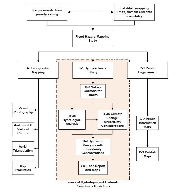
Figure 2.1 - General practices for flood hazard delineation.
Text version - Figure 2.1
Figure showing a graphical representation of the framework and outlines the general practices of a flood hazard delineation study.
As shown in Figure 2.1, after setting the study scope and determining the data sources, a flood hazard delineation study progresses in three paths: A) topographic mapping; B) hydrotechnical study, discussed in this document; and C) public engagement. The three paths are interlinked; and from the beginning, the interested parties and rightsholders need to understand the process for flood hazard delineation and its interpretation in an ongoing and transparent way, as the
public can provide valuable information to guide flood hazard studies based on local knowledge and priorities. The hydrotechnical study relies on information from the topographical mapping path. The design flood assessment needs to include current and future land uses and meteorological parameters before the hydraulic/hydrodynamic analyses, and the study has to consider the range of uncertainty.
The last step of the hydrotechnical studies path fully reports the results as shown on maps that are explained to interested parties, such as rightsholders, land-use planners, emergency officials, and the public, interlinking with the public engagement path. This third path needs to clearly explain the methods and uncertainty limits as well as possible mitigation measures for the flood hazard delineations so that all will understand them. Public information sessions, such as open houses, public webinars, and workshops, are possible vehicles where the practitioners may answer questions to help explain the flood delineation process more widely and these may occur throughout the study, not only at the end.
This document focuses on the hydrotechnical studies path. For guidance on the provision and dissemination of topographical mapping and geospatial data, one may refer to the Federal Flood Mapping Guidelines Series document titled Federal Geomatics Guidelines for Flood Mapping. Detailed guidance on engagement of rightsholders, interested parties, and the general public is available elsewhere.
The procedures for the hydrotechnical studies are presented in Figure 2.2.
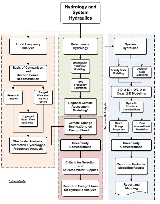
Figure 2.2 - Hydrology and system hydraulics procedures.
Text version - Figure 2.2
Flow chart showing the procedures forhydrotechnical studies
The design flow or water level assessment follows an initial flood frequency analysis (FFA) or an initial deterministic hydrology approach. It may use both as a verification of the calculations. The resulting range of design flow peaks or hygrographs are used in the hydraulic analyses to determine the depths and velocities and the range of flooding extent at the study site related to the probabilities of each peak flow or hydrograph. If necessary, the hydraulic analysis will also consider ice-related effects, wind, and wave effects, and/or geohazard effects to delineate the flood hazards to map.
The FFA approach looks at the historical streamflow or water level data, if available at that study site. If necessary, the approach synthesizes the data for the site allowing an analysis of the data. Synthesizing might involve removing the effects of regulating reservoirs. In ungauged regions, there will be a need for the hydrologic analysis to transpose historical gauged watershed data to the study site. The FFA path includes frequency and uncertainty analyses of the time series. Section 5.4 of this document describes the various types of flood frequency analyses and the procedures in more technical detail than given in Section 2.2.1. Based on the criteria for selection and available data, this approach ends with an evaluation of potential climate change implications on design floods, as described in Section 4.0. The results from these analyses may be compared to results from any previous studies, other methods in this approach or the results from the other approach, deterministic hydrology.
The deterministic hydrology approach uses a hydrologic modelling or geostatistical simulation for the hydrologic analysis. Both methods may define a design flow or a set of flows at a few probabilities. Section 5.5 of this document explains the use of these procedures in more technical detail than given in Section 2.2.2.
The flow frequencies estimated by the model may be compared to the series of flows estimated with a regional climate assessment model (Section 2.3 or technical details in Section 4.0). Approaches and procedures to account for climate change impacts in flood hazard analysis are evolving. Practitioners are encouraged to review recent scientific literature for the region of Canada where they are working. Some common approaches today include downscaled climate projections and deterministic hydrologic modelling using an ensemble of runs, which will help to determine the projected uncertainty range. Uncertainty derives not only from variable future climate conditions, but also from the numerous sources of uncertainty in the hydrologic simulation model (Section 9.0). As in the FFA approach, professional knowledge is required, and the qualified professional should compare the results with those from any previous studies or other methods and investigate the climate change and uncertainty implications on the design flows.
The resulting design flows are now ready for reporting before the next step of incorporation into the hydrotechnical study. The next step is to determine the extent, the depth, and, under the criteria of some jurisdictions, the velocity of flooding. A surface water profile model, either a steady-state dynamic model of constant peak flows or an unsteady-state dynamic model of design flow hydrographs simulates the hydraulics of the design flows. Section 6.0 of this document explains hydraulic models in more technical detail than given in Section 2.4.
The model may calculate the water depths in one dimension (1-D), that is, linearly along the main flow path of the watercourse. Alternatively, the model may calculate the water depths accounting for flow in two dimensions (2-D). Professional judgment and understanding of local hydraulic conditions are required to determine the type of hydraulic model being used.
Depending on the study site, the flood hazard delineation study may next consider ice effects (Section 2.5 or for further details Section 7.0), or lakeshores (Section 2.6 or the further explanation in Section 8.0). The study can then consider the uncertainty of the results—inherent in natural phenomena, stemming from uncertainties in the data, analytical processes, and the parameters used in the models—to define a range of values for the results, as explained in Section 2.7. Section 9.0 has more technical details. Finally, the study produces a report and results ready for mapping as described in Section 2.8. Section 10.0 provides the detailed requirements for a report that completes a quality-controlled flood hazard delineation study.
The following subsections explain the basics of each practice and Section 3.0 describes the data requirements in a general way for flood hazard delineations. Subsequent sections go into more detail on the technical procedures for flood hazard delineation.
2.1 Scope of Work Requirements
A scope of work description is included here to assist agencies that are contracting flood hazard delineation projects.
The study scope needs to clearly define the study site and the extent of the body of water. It should give the design flood criterion, as defined by the province or territory. The scope should also include an assessment of the potential impacts of climate change on the flood hazards in the area and recommendations on if and how these impacts should be accounted for within the study. The study scope should include an assessment, within accuracy bounds determined by study uncertainties, of how the identified design flood criterion will change over this timeline (e.g., change in vertical flood level for a 1% AEP event or change in AEP for a fixed vertical flood level). The scope needs to consider the flooding processes causing historical high-water events, such as whether the high water occurred from rain, snowmelt, wind and wave effects, ice-jam flooding, or some combination of these events. This will define the approach to the design flood assessment.
In many parts of Canada, processes leading to flood events are complex and often correlated, however this correlation structure may break down in a changing climate. Therefore, in some cases it is critical to consider joint probabilities rather than the product of individual probabilities (which would result in underestimating actual event probabilities). Section 5.4.6 covers the technical details of joint probability analysis in the hydrotechnical context.
The scope of work should clearly define the differing roles of those involved.
The scope of work needs to be commensurate with the funds available to undertake the work. An extensive study requiring detailed data is expensive and limited funds available thus dictate the priority and scope of studies. The land use of the areas under historical high water and potential economic consequences of flooding may be used to define the level of analysis.
Undeveloped areas may be less critical, while dense residential and institutional areas may require a finer resolution of the flood hazard delineation.
The study scope should include the objectives, context, and background information. Clear, specific information should be provided on the following aspects:
- Spatial extent
- Spatial resolution
- Data available and data gathering needs (Section 3.0)
- Community engagement
- Requirements for final reports and flood delineation maps
- Delivery milestone dates of the study components
2.2 Design Flood Assessment
After the collection of data elaborated in Section 3.0, the next procedure is to assess the design event (flow for open-water streams or water level for ice-related or lakeshore flooding) for the regulatory criterion of the jurisdiction of the study site. Hydrologic procedures are used to determine the design event. Figure 2.3 illustrates a sequence of the hydrologic procedures used to develop reliable and realistic design flood events for a given criterion, resulting in a report documenting the hydrologic analyses that have been undertaken.
The first step of the hydrologic analysis is, therefore, to define the flooding criterion, as specified by the jurisdiction, as one of the following:
- A single regulatory annual exceedance probability (AEP) event
- A series of events corresponding to a series of AEPs
- A meteorological event of given probability (intensity duration rainfall)
- A historical record event.
Section 5.1 discusses the design criteria in greater detail.
The second step is to determine the technique of the analysis for determining the value(s) for this criterion, such as a deterministic hydrologic simulation model and/or FFA, either single station or regional aggregates of observations. Later subsections in Section 5.0 go into the technical hydrologic procedures to assess the design event(s).
A climate change analysis, as explained in Section 4.0, is the next consideration in the process to obtain final design events that reflect both present and future environmental conditions. The hydrologic report presents the outcomes as peak events at various AEP or as hydrographs of flow over a certain duration (Section 10.0 details the requirements of the hydrologic report).
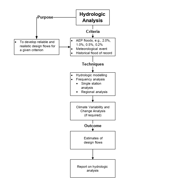
Figure 2.3 - Focus of hydrologic requirements in flood hazard delineation.
Text version -Figure 2.3
Flow chart showing the sequence of hydrologic procedures when creating a design flood event criterion.
Deciding what technique to use (refer to Section 5.3), including the process of identifying and implementing the appropriate hydrologic procedures, is often iterative. A preferred method may be identified, but later discovered to be infeasible due to insufficient data or because of external factors affecting the hydrology (e.g., land use/cover changes) during the period of record. In such cases, an alternative method may need to be implemented.
Figure 2.4 summarizes the considerations when determining which hydrologic technique to employ based on the needs of the design event and the uses, as well as the available data. The figure also indicates the criteria for the technique.
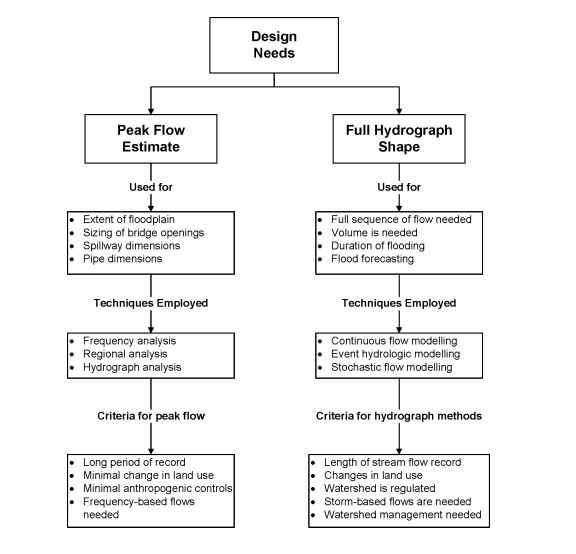
Figure 2.4 - Hydrologic design methodologies.
Text version - Figure 2.4
Flow chart summarizing considerations when choosing a hydrologic technique based on a design event.
Multiple procedures may be used to validate the results of the hydrologic study from the “preferred” procedure. For example, an AEP flow obtained from a hydrologic model can be verified by comparing the flow with corresponding results from a flood frequency analysis, by evaluating against known observed events, or by comparing the flow with the results from a regional model.
2.2.1 Flood Frequency Analysis
Flood frequency analysis (FFA) uses statistical techniques to determine the probabilities of a series of observed events, either instantaneous flows, daily flows, or water levels. The FFA requires hydrometric data of sufficient record length and reliability. A potential framework for frequency analysis, dependent on data availability, is shown in Figure 2.5.
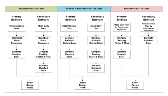
Figure 2.5 - Length of record constraints on hydrologic procedures.
Text version - Figure 2.5
Flow chart showing a potential framework for frequency analysis based on data from less than 10 years to over 25 year flow records.
Figure 2.5 indicates the primary and secondary hydrologic procedures a qualified professional would typically use depending on the length of recorded streamflow (or water level) data available. When a site’s sample size is too short, that is, the record length is less than recommended in Figure 2.5, the record can be extended by considering other data from similar watersheds or locations either within the study watershed, within the broader region containing the watershed or nearby water level gauges. Section 5.2 describes some possible approaches for extending the period of record and the process for handling regulated recorded flows. Section 5.4 describes flood frequency analysis, a common hydrologic method for both flows and water levels, in technical detail. Figure 2.5 also includes the use of a regional flood frequency analysis (RFFA) to determine the design event for the study site. Historical events may be compared to the results of the analysis for validation.
2.2.2 Hydrologic Modelling
Another common hydrologic method to determine streamflow is hydrologic modelling. Figure 2.6 shows the hydrologic modelling framework. It defines a hydrologic model, when to apply it, and what its uses are. A hydrologic model is often used to determine flows under future conditions of land use and meteorology or when insufficient observations exist for an FFA. It is specific to a watershed and requires parameters describing the physical terrain of the watershed. Section 5.5 describes hydrologic modelling in technical detail.
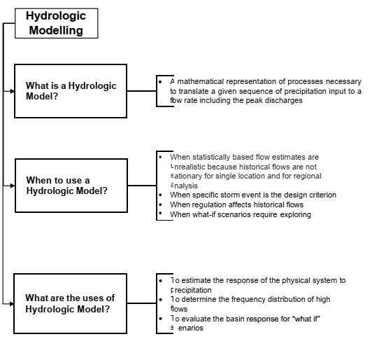
Figure 2.6 - Hydrologic modelling framework.
Text version - Figure 2.6
Flow chart describes a hydrologic model, when it should be used and what it can be used for.
Sections 5.5.2 and 5.5.3 explain when to use the various forms of these models. Design flows associated with a design storm input can be determined from single event models or continuous simulation models. Some models can also be used in either single event or continuous simulation mode. The simulation of snowmelt requires the model to include temperature as well as precipitation data. The development of every hydrologic model requires calibration and validation to observed sets of input and flows to ensure the best simulation of conditions. The model development process is detailed in Section 5.5.5.
2.2.3 Evaluation of Design Event
Whatever hydrologic approach is taken, whether a single station FFA, RFFA, an FFA of hydrologic model-produced data, or the data from a hydrologic model of a design event, the qualified professional should consider evaluating the results with those from a different technique, historical records, and results from nearby similar basins to determine that they are reasonable. Where possible, qualified reviewers not involved in the project should review the data, the methods, and the results.
Future land use changes will alter future flows because infiltration of the precipitation into permeable soils will change with land development. Evapotranspiration rates change with changes in vegetation cover. These changes result in differences to the peak flows of rivers. If these future changes are not considered, the responsible authority should realize that the lifespan of the resulting flood hazard delineation will be limited. Another cycle of mapping, starting with the design flood assessment, should occur after major shifts in land use.
Climate change is expected to shift some precipitation that traditionally came in the form of snow to winter rain, produce earlier freshets, and increase the intensity of rainfall. Mid-winter thaws also increase the likelihood of ice-jam flooding. As a result, climate change may also impact the design flood assessment.
2.3 The Influence of Climate Change on Design Flows
Future climate patterns, including those that directly and indirectly influence key national flood mechanisms, are projected to differ significantly from the historical record. The Atlas of Mortality and Economic Losses from Weather, Climate and Water Extremes (1970–2019) (WMO, 2021) shows that extreme weather events have increased from a baseline in 1970. From 1970 to 2019, weather, climate, and water hazards accounted for 50% of all disasters, 45% of all reported deaths, and 74% of all reported economic losses around the world. The rates increased considerably each decade over the initial decade 1970–1979 as the impacts of climate change intensified.
The first report to be released as part of Canada in a Changing Climate: Advancing our Knowledge for Action (Bush et al., 2019) discusses changes to Canada’s temperature, precipitation, and oceans, both change that has occurred and that may occur in the future. It explains how and why drought, wildfires, and extreme, intense rainfall are more likely in the future.
Two publications, “Canada in a Changing Climate: Sector Perspectives on Impacts and Adaptation” (Warren & Lemmen, 2014) and “Canada's Marine Coasts in a Changing Climate” (Lemmen et al., 2016) indicate that changing precipitation patterns under climate change may expose new areas to the effects of floods and may increase the magnitude and frequency of flooding in areas already impacted by flooding. However, not all locations in Canada will see increases in the magnitude and frequency of fluvial flooding under some climate change emissions scenarios (Gaur and Simonovic, 2018).
There currently is not a standardized engineering practice for assessing the impacts of climate change on flood hazards. However, assessments of flood risks to property and human life or safety benefit from considering the impacts of future flooding conditions under a changing climate both in inland and coastal situations. The complexity of this assessment is likely to be tailored to the project and as the engineering practice evolves.
2.4 Hydraulic Numerical Models
Hydraulic numerical models simulate the flow characteristics of depth and, in some applications, the velocities, of the design flow over the extent of the study site.
Figure 2.7 shows the purposes, inputs, techniques, and outcomes of the hydraulic analysis procedure.
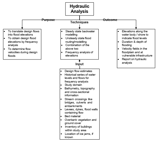
Figure 2.7 - Hydraulic requirements in flood hazard delineation.
Text version - Figure 2.7
Flow chart showing the purpose inputs, techniques, and outcomes of a hydrologic analysis procedure.
2.4.1 Flood Fringe
An important concept that has been adopted by some jurisdictions as part of land-use planning in areas that may be subject to flooding is the division of the flooded area into the floodway and flood fringe. While exact definitions vary across Canada, the floodway is generally the area where flows are deepest, fastest, and most destructive; the flood fringe is generally shallower and has slower velocities than in the floodway. The flood fringe may be inundated under the design flood but would not be subject to hydraulic conditions that make mitigation measures impractical nor cause significant negative impacts on the flood levels and velocities of adjacent areas. New development in the flood fringe may be permitted in some municipalities depending on local guidelines, which vary by jurisdiction.
Some jurisdictions in Canada define the flood fringe as regions of the floodplain where encroachment will not result in an increase in water levels in the floodway. In other jurisdictions, the flood fringe may be defined as a combination of water depth and velocity. This definition does not take into account the potential impact of encroachment on water levels.
To produce the hydraulic parameters necessary to define the floodway and flood fringe requires specific configurations of the hydraulic models used to produce inundation maps, as explained in Section 6.0.
2.4.2 Modelling Dimensions
Most hydraulic models are based on the finite difference solution of equations for either one- dimensional (1-D), two-dimensional (2-D), or three-dimensional (3-D) fluid flow. These equations define the principles of conservation of mass and momentum balance in a fluid. They are sometimes simplified in hydraulic models to exclude various terms in the equations. When the calculations consider the flow in only one direction along the channel stream, the model is 1- D and can determine the water surface elevations at various cross-sections of the stream. When the calculations consider the flow in two horizontal directions, the model is 2-D. Although a 2-D model can determine water levels and velocities, it requires more detailed bathymetry of the channel and the surrounding terrain (e.g., LiDAR topography). A 3-D model considers the flow in three dimensions, the two horizontal and the vertical.
Most riverine flood modelling in Canada is carried out using 1-D models. 2-D models are used for more complex situations (e.g., overland flows, lakeshore flooding, etc.) or when detailed velocity information is desired. Table 2.2 provides some general situations and recommended approaches to hydraulic model selection that may be considered for flood mapping purposes.
| Suggested Approach | Situation |
|---|---|
| 1-D Modelling | Length of channel-to-flood-hazard-area width ratio larger than 3:1 |
| Rivers and flood hazard areas in which the dominant flow directions and forces follow the general river flow path | |
| Steep streams that are highly gravity-driven and have small overbank areas | |
| River systems that contain a lot of bridges/culvert crossings, weirs, dams and other gated structures, levees, pump stations, etc. and these structures impact the computed stages and flows/velocities within the river system | |
| Medium to large river systems, where model includes a large portion of the system (> 150 km) | |
| Areas in which the basic data does not support the potential gain of using a 2-D model | |
| 2-D Modelling | When modelling an area behind a system of berms, levees, or dikes, and where the water can move in many directions, non-parallel to the main river, if the system is overtopped and/or breached |
| Bays and estuaries in which the flow will frequently move in multiple directions due to tidal fluctuations and river flows coming into the bay/estuary at multiple locations and times | |
| Areas and/or events in which the flow path of the water is not completely known | |
| Highly braided streams | |
| Alluvial fans | |
| Flow around abrupt bends | |
| Very wide and flat flood hazard areas, such that when the flow spills out into the overbank area, the water may take multiple flow paths and have varying water surface elevations and velocities in multiple directions | |
| Applications where it is especially important to obtain detailed velocities for the hydraulics of flow around an object, such as a bridge abutment or bridge piers, etc. |
2.4.3 Model Evaluation
A hydraulic (or hydrodynamic) model consists of the channel and/or shoreline geometry, including structures, and boundary water level conditions. As well, it has variable parameters, such as the roughness and hydraulic coefficients. The flows, water levels, and ice conditions of the design event(s) are the various scenarios that the model will simulate.
As with any model (e.g., hydrologic, climate, hydraulic, or hydrodynamic) the qualified professional should validate the results before analyzing the design event(s). After a sensitivity analysis of the parameters in the model, to see which parameters have the most significant change to the results, the modeller should simulate observed events to compare with the corresponding observed conditions. The parameters that simulate the observed conditions should be set in the model for the simulation of the design flow(s). As explained in Section 6.3, two sets of observations define a calibration and validation set that confirms the parameters work for a range of observations. Both sets should contain high flow conditions whenever possible.
Section 6.0 provides the technical procedures for hydraulic numerical modelling, including data requirements, a more detailed description of models, selection methods, verification, and reporting requirements specific to the hydraulic report.
2.5 Ice-Related Flooding
Many rivers and lakeshores in Canada are subject to ice-related flooding, requiring specific analyses for these circumstances in the flood hazard delineations. Climate change may change the incidences of ice-related flooding as winters get warmer, and ice forms later and breaks up earlier. Mid-winter thaws may become more likely and ice may be thinner and more likely to fragment and jam. A flood hazard delineation for rivers susceptible to ice jams requires modifications to the hydrology and hydraulics procedures, detailed in Section 7.0. Section 8.0 discusses ice-related flooding on lakeshores.
Analyses of rivers that have a documented history of ice-related flooding should include an assessment of the impacts of ice jams on water levels and AEPs. Rivers that may not have a documented history of ice-related flooding, but have characteristics that may lead to ice jams, should be evaluated for ice-jam risk.
The conditions that influence the formation of ice jams include:
- Water levels at freeze-up
- Channel characteristics, particularly known lodging points
- Characteristics of ice cover
- Breakup regime (thermal or mechanical)
- Characteristics of flowing ice
- River discharge
There are three main stages in the life cycle of river ice: ice formation, ice thickening, and ice breakup. Figure 2.8 identifies the ice-jam potential during each of the three different stages.
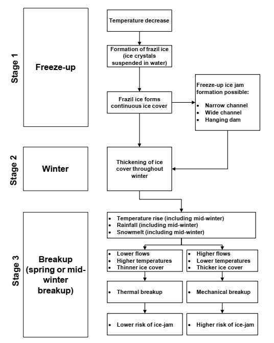
Figure 2.8 - Typical processes leading to ice jams.
Text version - Figure 2.8
Flow chart identifying the three life cycle stages of ice formation along with their ice-jam potential during each stage.
The primary cause of ice-related flooding in Canada is ice jams, which can occur at freeze-up, at breakup, or during a mid-winter thaw. Modelling ice-related flooding is a specific technical discipline, requiring the involvement of experts (Kovachis et al., 2017; Lindenschmidt et al., 2018).
2.6 Lakeshore Flooding
Areas on the shores of lakes may be flooded due to elevated water levels driven by hydrologic (water balance) processes, strong winds (storm surges), wave effects, and ice shove. Section 8.0 provides an overview of the procedures for lakeshore flood hazard analysis, incorporation of climate change impacts, and mapping lakeshore flood hazards. Guidance on procedures applicable to marine coasts is provided in the Federal Flood Mapping Guidelines Series document titled, Coastal Flood Hazard Assessment for Risk-Based Analysis on Canada’s Marine Coasts.
2.7 Uncertainty of the Flood Hazard Delineation Results
The physical processes involved in assessing design events are inherently complex and uncertain. Additionally, uncertainty stems from the methods and limits associated with the estimation of flood extents and depths. Therefore, flood hazard maps are subject to uncertainty. Uncertainty derives from the following four characteristic categories:
- Natural or intrinsic uncertainty from the inherent randomness of natural processes, which is variable over time and space. This natural uncertainty is difficult to reduce and quantify as the data is irreproducible.
- Data uncertainties from measurement errors, instrumentation errors, inconsistencies and non-homogeneity of the data, data handling, and inadequate representativeness of data over time and space. This data uncertainty may be reduced with better or increased measurements.
- Calculation uncertainty from the inability of a mathematical technique or model to accurately represent the true physical behaviour of the natural world, since the technique or model is poorly or incompletely specified, or the phenomena modelled has instabilities and non-linearities not reflected in the modelling approaches.
- Parameter uncertainties from inevitable inaccurately assessed parameter values in the test or calibration data, due to limited numbers of observations, and statistical imprecision.
These uncertainties should be acknowledged, and where appropriate, quantified, and managed.
These categories of uncertainties are interdependent and overlap as in the Venn diagram of the overall uncertainty space, shown in Figure 2.9. The overlap from the interdependencies reduces the overall uncertainty. An example of the interdependence is how the natural uncertainty impacts the measurement of water levels, which in turn reduces the certainties of the parameter valuation. Having uncertain values for the parameters means the model is uncertain. Thus, the quantification of the uncertainty is not the simple sum or product of the uncertainty of each but needs to also account for their interdependence. The flood hazard delineation results are uncertain because of the randomness of nature, the uncertainties of the data measurements, the models adopted for use, and the approaches used to estimate their parameters.
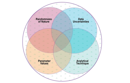
Figure 2.9 - Elements of overall uncertainty.
Tet tversion - Figure 2.9
Venn diagram showing the elements of overlap of flood hazard delineation results
- Randomness of nature
- Data uncertainties
- Paramerter Values
- Analytical technique
Section 9.0 describes some approaches to address uncertainty in assessing flood scenarios, incorporating climate change, and the use of hydraulic models. Section 9.3 warns that changes in climate and land use can cause hydrologic, hydraulic, lakeshore, and ice assessments (and the flood hazard maps they support) to become obsolete. The periodic review of modelling assumptions is particularly important where flood hazard maps form the basis for flood risk planning and regulation, as discussed in Section 9.3. Documentation and data maintenance aids the periodic review of adaptive management. Adaptive management requires periodic reviews and points to the need for updates when they become necessary.
2.8 Report Details
As the work on a flood hazard delineation study progresses, the documentation should follow. Technical reports for the study site, as stipulated in the scope of work, may discuss in detail:
- Regulatory criterion
- Purpose of study (land-use zoning, emergency management, etc.)
- Data used
- Hydrologic procedures used and why they were selected
- Climate change assessment methodology and recommendations
- Hydraulic procedures used and how they were verified
- Any ice-related, wind set-up, and wave analyses
- Uncertainty of the results
- Reference to previous maps and models and any changes
- How the comments of the reviewers were addressed
Using the reports, another qualified professional should be able to recognize the procedures and use the data to replicate the results. The models and data should be provided so that when an update is required, the new data may be incorporated to update the flood hazard delineation. Section 10.0 lists the requirements for the survey and base data, hydrology, hydraulics, ice, wind, and wave effects.
2.9 Summary of General Practices
In summary, a flood hazard delineation study starts with a defined and clearly understood purpose and regulatory criterion. The technical work will not occur in isolation from communication with the interested parties, Indigenous rightsholders, communities, and the public. Communication occurs initially to help define the purpose, and subsequently to obtain data, explain procedures, and share results. The qualified professionals, following a scope of work designating the extent, criterion, and reporting requirements, will use hydrologic procedures to assess the design events and assess potential climate change impacts.
Hydrodynamic procedures will define the flood hazards for the design events. The hydrotechnical procedures may need to consider ice-related or coastal (wind and wave) effects at certain study sites that see these flood impacts. Before the final reporting of the flood hazard delineation, the qualified professionals will address the uncertainty of the results.
All of these procedures rely on high-quality geospatial, hydrometric, meteorological, and non- systematic data as explained in the following section on data requirements.
3.0 Data requirements
The flood hazard delineation study relies heavily on multiple sources of data. However, data availability will restrict the type of analysis possible. Data inform the approach taken in every stage of the analysis, from the design event assessment to the hydraulic flow analysis, to the considerations for ice, wind, and wave effects and other factors influencing flood hazards. The quality of the data affects the quality of the results. This section details the various data required for the hydrotechnical procedures that support a flood hazard delineation study (see Figure 3.1). The following sections provide sources for geospatial, hydrometric, meteorological, and non- systematic data, as well as brief explanations of how these data are used in the analysis. Each section on a particular procedure goes into more depth on what data are required for that procedure and how they are used.
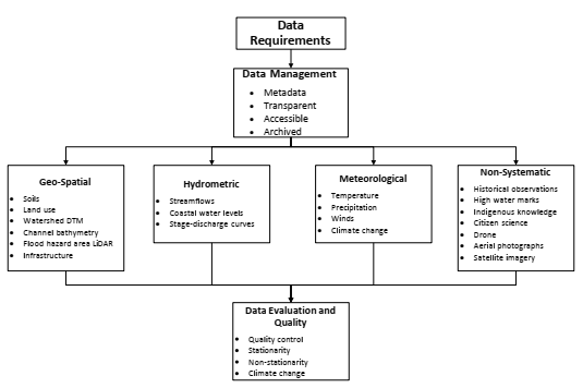
Figure 3.1 - Data requirements for flood hazard delineation.
Text version - Figure 3.1
Flow chart showing data requirements for flood hazard delineation.
3.1 Data management
Data management is integral to the flood hazard delineation procedures. Not only does the data need to be of high quality, but the study participants and interested parties need to know the source and methods of collection, known as the metadata. Wherever possible, the data should be open and transparent so that everyone has access to the data, at least from the original sources. Indigenous knowledge should be collected, protected, used, and shared according to the First Nations principles of ownership, control, access, and possession (OCAP®)—see Section 3.5.2. Collaboration among First Nations, Inuit, Métis, academia, other government agencies, and consultants increases when the data is easily transferable and open. The archiving of the data is also important to maintain the life and reproducibility of the flood hazard delineation results into the future. The study archive should maintain a copy of the actual data used in the flood hazard delineation study. Permanent data held by other agencies, such as national hydrometric data, may be cited, recognizing that data links may change over time, as do data of dynamic processes. Section 10.0 describes the details to include in the report on the collection and maintenance of data for the flood hazard delineation study.
3.2 Geospatial Data
Hydrotechnical procedures require geospatial data, including watershed areas, surface water networks, topographic data, watershed slopes, stream slopes, bathymetry, stream cross- sections or bathymetry, lake areas, land use coverage, infrastructure, and other hydrologic features. Geographic information systems (GIS) may store the data in easily accessible layers linked to tables of the data. The accuracy and precision of flood hazard maps are highly dependent on the quality of the geospatial data used.
3.2.1 Surface Water Network
The delineation of surface water networks and watersheds may use NRCan’s National Hydro Network (NHN) data model (NRCan, 2019) to provide geospatial digital data of lakes, reservoirs, rivers, and streams.
3.2.2 Soil Data
Soil data for the watershed under study, in particular its permeability, plays an important role both in hydrologic models and in RFFA to move point data to similar watersheds. General classifications of soils are available in GIS layers, such as Global Soil Datasets for Earth systems modelling (GSDE), or hard-copy maps by provincial agricultural agencies. The soil classifications may help determine the rate of infiltration of snowmelt and rainfall in each area of the watershed.
Furthermore, the bed material of a channel or water body will affect the hydrodynamics of flow, so the qualified professional will require knowledge of the bed material: coarse or fine sand, silt, gravel, or cobbles. Soil data is also invaluable for geomorphological analyses studying the shift of stream beds, and for geohazard studies analyzing the risks of slumps, landslides, and debris flows.
3.2.3 Land Use Data
Land use data, which shows the predominant land cover in the watershed, whether high-density development, low-density construction, vegetation, forests, or industrial activities, such as strip mines, plays an important role both in developing hydrologic models and in regional flood frequency analyses to translate data between similar watersheds. Generally, higher density areas with impermeable surfaces will generate more runoff quickly since less precipitation infiltrates into the ground.
In addition to current land uses, consideration of future land use and probable land cover is important to ensure the longevity of the flood hazard delineation mapping. Lowland areas of an urban area, developed according to flood hazard maps, may be subjected to regular basement flooding because the sewer system is now unable to handle the increased intense runoff from later suburban development in the previous agricultural areas upstream. Forest fires, insect infestation, or arboreal disease may clear large tracts of forest, which can decrease the permeability, infiltration, and evapotranspiration of that portion of a watershed. This results in increased runoff and risks of mud and debris flows in steep watersheds. Poorly managed logging and clearing swaths within forested watersheds can have the same effect. Other industrial activities, such as mining, also impact runoff and flood hazards. Drainage or loss of wetlands, marshes, and bogs can greatly impact the flooding characteristics of a watershed, since wetlands attenuate peak runoff, storing the water for later release, among other ecological benefits.
Recent topographical maps, GIS data (e.g., Commission for Environmental Cooperation, 2020), aerial photography, and city zoning data provide high-quality land-use data at fine resolutions. Future land uses incorporated in municipal, provincial, and territorial legislation, approved and proposed development plans, and zoning codes and bylaws are a source of planned land use changes. Unplanned land use changes, such as forest fires, pests, and arboreal disease are unpredictable and introduce uncertainty into the flood hazard delineations where they occur.
3.2.4 Topographic and Bathymetric Data
The digital terrain model (DTM) of the study watershed is important not only for the design flow assessment but also for routing the flow down the stream channel, estimating wave uprush, and mapping areas of lakeshore flooding. The Federal Airborne LiDAR Data Acquisition Guideline (NRCan & PSC, 2018) and the Federal Geomatics Guidelines for Flood Mapping (NRCan & PSC, 2019) provide guidance on sourcing and using LiDAR. LiDAR flights collecting river and lakebed bathymetry data should be flown at the lowest water level possible. Bathymetry may be collected by sonar surveys by boat. The resulting data from the two collection methods should mesh along the water’s edge to describe the terrain under a full range of water levels.
The GIS layer of the DTM for the watershed, compiled from topographic maps, local GIS, orthophotography and available LiDAR, is important in hydrologic models as it will define the extent of the watershed, the slope and aspect of the watershed’s water courses, and their locations. These parameters are also required to determine the hydrologic similarity of watersheds above gauging stations.
The hydraulic models that will estimate the extent, depths, and velocities of the design floods require nearshore topography (e.g., LiDAR) and bathymetry of the channel beds and flood hazard areas. The availability of this data will often determine the choice of hydraulic model and may require field surveys to obtain the necessary details for a geo-mesh or cross-sections of the channel and flood hazard areas.
3.2.5 Infrastructure Data
Infrastructure, such as reservoirs, tailings ponds, stormwater management ponds, culverts, bridges, berms, embankments, and dikes, influences streamflows and water levels. The relationships of stage (water elevation), storage volume, and discharge for reservoirs, tailings ponds, and stormwater ponds are required to assess the parameters for hydrologic routing or hydraulic routing models to determine the design flow. Record drawings or field surveys showing the size of culverts and bridge piers, distances between bridge piers, revetment of berms, embankments, and dikes allow the hydraulic models of the stream channel to determine the extent, depth, and velocities of flooding.
3.3 Hydrometric Data
Hydrometric data is a key systematic data requirement in establishing the design flow. It includes instantaneous and mean daily stream discharges and water levels measured at hydrometric stations.
3.3.1 Streamflows and Water Levels
Hydrometric data availability is fundamental to choosing appropriate hydrologic procedures and to the output of accurate hydrologic design streamflows. Hydrometric data is the basis for FFA and is also integral for the verification of hydrologic and hydraulic models. Water levels may form the boundary conditions for hydrodynamic models.
Additional to the gauges on the study stream, the hydrologic procedures may use gauges from a hydrologically similar region; for example, studies on ungauged streams will generally include data from neighbouring gauged streams in similar watersheds. A watershed is hydrologically similar when it has a similar precipitation, size, slope, orientation, and land cover. A neighbouring watershed is not similar if it does not meet these characteristics and the data should be used with caution. A regional regression analysis may develop a relationship with these factors and gauged streamflows within the region to estimate streamflows at ungauged sites.
Hydrometric data in Canada is available from the Water Survey of Canada (2023), provincial agencies, and other sources, such as hydroelectricity generation facilities and private companies. Potential sources of hydrometric data should be researched. Record the station metadata including the following:
- Location
- Length of record
- Regulation type
- Period of record
- Datum
- Data provider
- Operation schedule (e.g., continuous, daily)
- Discharge conditions (e.g., under ice, at breakup, affected by beaver dams, vegetation, etc.)
- Remarks (e.g., records being reviewed)
- Drainage area upstream of the gauge
3.3.2 Tidal Water Level Data
Measured water level data and tidal constituents may be required for flood delineation studies near marine coasts. Data is available from the Canadian Hydrographic Service (CHS, 2021b), which maintains a network of stations along Canada’s marine and Great Lakes coasts. The Water Survey of Canada also maintains a network of inland lake stations.
The data is typically used to examine historical storm surge events, determine tidal planes, and support numerical modelling efforts. For riverine flood studies, the sea level acts as a downstream boundary condition that influences water levels in the river.
3.3.3 Stage-Discharge Relationships
Hydrometric technicians develop stage-discharge relationships whenever observed water levels (stage) are used to obtain flow (discharge) estimates at a site. Generally, when published streamflow data are available, a stage-discharge relationship will also be available from the same source. Reviewing changes in relationships over time is helpful in understanding uncertainties in the flow data, as is identifying the degree of extrapolation from the most extreme measured flow.
Establishing a new gauging location or estimating discharges from miscellaneous water level data (see Section 5.2) requires the development of a new stage-discharge relationship. Measurements of flow and depth, as well as the “curve fitting” required in developing the relationship, require skill and are subject to uncertainty.
Stage-discharge relationships are typically specific to open water flow and may change with time or become irrelevant under ice-jam conditions, shifting beds, or changing vegetation or debris conditions. Relating stage to flow under the condition of high flows can be particularly uncertain due to extrapolation, gauge loss or damage, overtopping or breaching of flood defences, and, in extreme cases, avulsion that changes flow paths within the stream channel or flood hazard area.
The design flow assessment procedures, the hydraulics procedures, and ice-jam analyses may rely on open water and ice-covered stage-discharge relationships, as discussed in the relevant sections.
3.4 Meteorological Data
Meteorological data may be required in procedures to estimate future streamflows under climate change and for simulation methods, such as hydrologic, ice, storm surge, and wave modelling. The meteorological data include rainfall, snowfall, barometric pressure, temperature, evaporation, number of days above/below zero, wind, and other data. Reliable meteorological data are necessary for hydrotechnical analyses.
3.4.1 Historical Temperature and Precipitation Data
Historical meteorological data are available for download on an hourly, daily, or longer time step from ECCC for 8,737 stations across Canada, including approximately 1,566 active stations (ECCC, 2021a). Other sources of meteorological data that may not be integrated into the ECCC database can include provincial governments, local and regional municipalities, conservation/watershed authorities/districts and other water management entities, environmental non-governmental organizations (NGOs), and citizen scientists.
Hybrid products of interest may be the Canadian Precipitation Analysis (CaPA) product. These data can be used as meteorological forcing for larger-scale hydrologic models and provide a robust interpolated gridded product.
Radar-rainfall data is useful in identifying the spatial distribution of rainfall events. This can be particularly helpful when calibrating and validating hydrologic models for specific rainfall events. Snowpack data including snow depth, density, and water equivalent are frequently required for hydrologic modelling. Current measurement networks are relatively sparse due to the expense and complexity of widely used in-situ instruments, although this situation may improve with new low-cost remote-sensing technologies (see Section 3.5).
The purpose of using a historical storm event in the computation of floods is to generate simulated flow for a specific event. Several storms and rainfall distributions may also be developed to generate simulated flow, as explained in Section 5.5.
3.4.2 Climate Change Monitoring Network and Model Data
ECCC maintains a multi-decadal climate monitoring network and has participated in coordinated climate modelling exercises that have enabled the production of climate change scenarios for Canada and at the global scale. Recently, ECCC established the Canadian Centre for Climate Services (CCCS) to increase access to regional climate information, data, and tools that may be useful to support flood hazard delineation procedures. Additional regional climate information includes sources such as Ouranos, ClimateWest, and the Pacific Climate Impacts Consortium (PCIC), as well as regional academia and consultants.
3.4.3 Intensity Duration Frequency Curves
Intensity duration frequency (IDF) curves provide input to hydrologic models, many in the urban context, relating local rainfall patterns to a design AEP. IDF curves for select sites are available from ECCC, derived from recent precipitation data (ECCC, 2021b). IDF curves may be adjusted to reflect changes in rainfall intensity due to climate change using established procedures (CSA, 2019; ClimateData.ca, 2022).
3.5 Historical Non-Systematic Data
Historical records provide sporadic details that may be used to augment the systematic hydrometric record (see Section 5.2.4) and provide coincidental data for hydrologic, hydraulic, ice, and storm surge model verification. In many locations, the historical water levels become the regulatory flood hazard line. In some jurisdictions in Canada, the entire flood hazard areas are defined, and development guided, to historically based flood lines. Additionally, there are computer programs that allow the input of non-systematic information to adjust frequency-based flow analyses. Historical records include newspaper and video media accounts, and records from churches, RCMP, municipal emergency officials, and archived Hudson Bay officials’ journals. As well, other non-systematic data sources are also available, as outlined in the following subsections.
3.5.1 High-Water Marks
High-water marks are physical evidence of flooding extent, including debris, sediment deposits, staining, scars on trees, and water damage. Survey crews can document this physical evidence to determine approximate flood extent and depth; however, it may not always be possible to determine the precise time of maximum flooding or the corresponding maximum discharge. In some incidences, historical high-water marks have become the regulatory high-water levels.
3.5.2 Indigenous Knowledge
In many watersheds, Indigenous communities have knowledge of high-water events, ice-jam formation processes, and flow–land use relationships.
When collaborating with Indigenous communities, any data or information about Indigenous communities should be collected, protected, used, and shared according to the First Nations principles of ownership, control, access, and possession (OCAP®) (First Nations Information Governance Centre, 2022). If Indigenous knowledge is communicated through the project to a broader audience, communication should align with the wishes of the Indigenous communities involved.
3.5.3 Citizen Science
Mobile phones produce high-resolution photographs that are typically time-stamped and geo- referenced. Citizens may photograph and record videos of flooded areas, which can be interpreted by practitioners to determine flood extents. The utility of the data in hydrologic procedures will depend on the ability to translate the observations into water level estimates. Rivers and shores may be very dangerous areas, particularly during flood events, so citizens are encouraged to remain well away from banks, shore structures, and bridges.
Several initiatives in Canada are engaging citizen scientists, primarily by gathering and submitting environmental and ecological data via mobile phones and the internet. Current examples include earthquake reporting through Natural Resources Canada (NRCan, 2017), and the Agroclimate Impact Reporter from Agriculture and Agri-Food Canada (AAFC, 2017).
In the United States, the National Oceanic and Atmospheric Administration’s (NOAA) Meteorological Phenomena Identification Near the Ground (mPING) project (NOAA, 2017) has produced a mobile app that enables citizen scientists to submit reports on meteorological and physical events, including rain, snow, mudslides, and flooding. The data is then filtered and used to ground-truth satellite observations.
Additional sources of usable data include social media posts and photograph or video sharing about flooding events and other disasters. There are also initiatives to correlate the prevalence of certain words, terms, and tags to the progression of on-ground conditions; however, separating legitimate signals from invalid ones is challenging, requiring robust quality assurance methods. Accurate water level and discharge estimates must be derivable for the data to be useful in hydrotechnical procedures.
Snow depth measurements with comparable accuracy to meteorological station instruments are now routinely derived from remote web-camera imagery of rulers placed in snowpacks. This measurement concept allows for a large number of measurements from remote locations and can leverage camera networks used for other monitoring purposes, such as security, habitat, recreation, and transportation.
3.5.4 Autonomous and Remotely Controlled Aerial Vehicles
Autonomous and remotely controlled aerial vehicles are either fixed-wing or rotary-wing aircraft that are flown without a pilot present on board and are also commonly referred to as unmanned aerial vehicles (UAVs) and drones. These aerial vehicles can either be flown using a pre- programmed routine or behaviour, or by a pilot flying the aircraft remotely by sight or instruments. UAVs are excellent tools for monitoring flood conditions and providing high- resolution, time-stamped, and geo-referenced images for post-flood model calibrations and for determining flood extents. They are also useful for other data collection purposes, such as identifying watershed land use and creating high-spatial-resolution maps of depth change.
3.5.5 Aerial Photographs
Aerial photographs and orthophotography are another valuable tool in preparing data for use in hydrologic and hydraulic modelling (e.g., identifying the extent of different types of land use).
Many provinces and territories have flown portions of their jurisdictions at periodic times and aerial photographs may be available for the study location over a multi-decadal range of time. In addition, NRCan’s National Air Photo Library contains over 6 million aerial photographs covering all of Canada, with some photos dating back to the 1920s.
Morphological changes visible in aerial photographs provide an approximation of the sensitivity of sediment aggradation or erosion to peak-flow events. Aerial photographs can also be used to identify geomorphological changes in watercourses over time. Orthophotography aids in identifying flood extents for actual events to derive water levels paired to discharges for use in hydraulic model calibration.
3.5.6 Satellite Imagery
Satellite image analysis is a practical way to determine floodwater extent at different times and land use. Canada’s RADARSAT-2 satellite is capable of providing spatial resolution of 1 m and data is available through MDA Ltd. (2021) for commercial clients and the Canadian Space Agency (CSA) for federal government clients (CSA, 2021). Satellite images can be acquired, received, processed, and delivered based on client requirements. RADARSAT-2 data are excellent for delineating flood extents to provide model calibration points.
3.6 Data Evaluation and Quality Assurance/Quality Control
The flood hazard delineation procedures are only as accurate as the geospatial, hydrometric, meteorological, and non-systematic data used. The quality of the data and the incorporation of sound procedures and judgment are all vital elements in generating robust and successful outcomes. Careful evaluation of data quality prior to use is necessary due to the wide variations in data quality that exist, and depending upon the data source, the condition under which these data were collected, and many other factors.
All systematic data must be subject to a quality assurance and quality control (QA/QC) process that includes, at a minimum, screening for:
- Missing data
- Outliers or suspect data
- Data jumps or broken lines
- Data flags
A description of how missing or unreliable data was managed must be included in the study report. Additional information on QA/QC is included in Section 5.4.3.
Historical and other non-systematic data may be included in analyses using a threshold of perception approach, described in Section 5.2.4. Care must be taken, as the reliability of the data may be suspect. However, the data provides a guide to the range of possible limits of the flood hazard delineation.
3.6.1 Stationarity
For many statistical analyses, such as flood frequency analyses, the data must be homogenous (e.g., drawn from one parent population), stationary (without trends or jumps), and without patterns, for the resulting probabilities to be valid. The stationarity of hydrotechnical datasets is typically impacted by any construction of reservoirs, removal of dams, land use changes, development (e.g., urbanization, deforestation), erosion/aggradation, climate change effects, or other factors. Therefore, an evaluation of the data requires knowledge of basin conditions over time in conjunction with a visual and statistical assessment for data stationarity at the beginning of all hydrotechnical procedures. Many statistical tests exist to assess the homogeneity and stationarity of data.
Qualified practitioners with expertise in advanced statistical flood frequency analysis methods that deal with heterogeneous and non-stationary data may employ these analytical tools to continue with a flood frequency analysis. One advanced process for heterogeneous data entails disaggregating the data—performing separate frequency analyses on each component before a recombination of the probabilities.
The effects of a changing climate may also have an impact on stationarity, as described in more detail below.
3.6.2 Land Use Changes, Development, and Morphology Non-Stationarity
Land use and development changes that can affect the stationarity of streamflow and flooding data include:
- New urban development, including sewers, paving, and construction.
- New agricultural drainage network development.
- New or altered flood mitigation measures, including dams (and their operation), dikes, berms, and conveyances.
- Changes within the stream channel, including to culverts and bridges, and morphological changes, such as erosion, aggradation, and channel alignment shifts.
- Anthropogenic (human-caused) changes to land cover that may alter interception, infiltration, evapotranspiration, flow routing, erosion, and sedimentation (e.g., timber harvesting, drainage of wetlands, and open-pit mines, etc.).
- Natural processes, including the effects of forest fires, parasites, and disease on vegetation.
Morphological changes affect the channel bed and banks, as well as the banks of larger bodies of water. Continuous erosion incrementally varies the hydrodynamic factors that impact flood hazard delineation, while catastrophic erosion, caused by the high water levels of a flood event, may dramatically impact the flood hazard delineation. Aggradation, the deposition of sediments at sections where the water flows more slowly, gradually builds up sand bars and beaches. The geometry of the channel or lakeshore bluff influences the dynamics of the design flow event. When the geometry changes, the depths and extents of flooding will also change. These morphological impacts may significantly influence the stationarity of the data.
3.6.3 Climate Change Non-Stationarity
Climate change is causing observationally detectable changes to meteorological conditions at global and regional scales, and these changes are expected to continue. As a result, climate change is and will become increasingly reflected at local scales in flood-relevant climate conditions. For example, changes in spatial and seasonal patterns of temperature, precipitation, and other climate variables may increase or decrease the magnitude and frequency of floods and expose historically low-flood-risk areas to flooding (Warren & Lemmen, 2014). In addition, climate change effects include reduced lake and sea ice, melting glaciers, and thawing permafrost (Warren & Lemmen, 2014).
Climate change effects may be difficult to detect within historical-based individual streamflow record data due to relatively short data collection periods and the high degree of natural variability in hydrologic variables. Hydrologic analyses should make appropriate allowances for climate change non-stationarity where trends are detected. Whether or not a climate trend or signal has been detected, a precautionary allowance may be appropriate (EGBC, 2017) and analyses can make use of climate change projections (see Section 4.0).
3.7 Summary
In summary, the quality of the flood hazard delineation study can be no better than the quality of the data used in the analysis. The sourcing and collection of good quality data are paramount. A sound data management approach is necessary to maintain the geospatial, hydrometric, meteorological, and non-systematic data components in an open and transferable manner between partners and interested parties. Any analysis done should be repeatable with those same data. Data control ensures the quality of the data, and the archived data should follow the reporting requirements listed in Section 10.0.
4.0 Incorporation of Climate Change
The intersection of climate change and the identification of flood hazard areas is an evolving issue. There are several issues that need to be addressed strategically by separating policy implications from the technical procedures. One area that may emerge beyond these guidelines is the management of the increased risk and the flood fringe zone between current and climate change–influenced flood zones. These guidelines are, however, limited to examining the technical procedures.
Another key aspect of incorporating climate change in the development of future flood hazard maps is the approach for addressing this. The current flood hazard mapping procedures may be applicable for small and medium basins or sub-basins, such as mapping of small but important stretches of a stream, areas of potential growth, etc., but current procedures to evaluate climate-induced impact are not advisable for these smaller areas. Rather, consideration should be given to regional/provincial climate change studies that will develop estimates for climate- induced hydrologic changes in terms of flow and timing of peak flows that are mapped for the entire region.
Integrating future climate conditions into flood hazard delineation is a challenge that has been applied in multiple jurisdictions across Canada and in other countries using different qualitative (e.g., adding “freeboard”, a vertical distance applied to account for uncertainty) and quantitative (e.g., modelling) approaches. The first volume of Case Studies on Climate Change in Floodplain Mapping was published in 2018 as part of the Federal Flood Mapping Guidelines Series (NRCan, 2018). This document includes three quantitative approaches used in different jurisdictions in Canada to incorporate climate change projections into flood hazard delineation. A second volume of case studies that incorporate climate change effects into flood hazard delineation is in the planning stages.
An Inventory of Methods for Estimating Climate Change-informed Design Water Levels for Floodplain Mapping (Khaliq, 2019) describes several approaches to quantify the impacts of future climate on flood hazards in Canada.
With each iteration of Intergovernmental Panel on Climate Change (IPCC) reports, the climate change projections are continually being updated, revised, and strengthened. Such changes result in an upward or downward adjustment of flood flow and flood level estimations. With improvements in techniques, the calculated uncertainty related to the impact of climate change on flood levels may decrease over time. One way that the uncertainty associated with various climate change scenarios and models can be quantified probabilistically is by using an ensemble approach.
Environment and Climate Change Canada (ECCC) has maintained a climate monitoring network for several decades and has conducted climate modelling that enables the production of climate change scenarios as part of global collaboration. Similarly, regional consortia, such as Ouranos in Québec (www.ouranos.ca), and the Pacific Climate Impact Consortium (PCIC) in BC (pacificclimate.org), have also developed regionally downscaled and bias- corrected derivatives of global climate model results. Recently, ECCC established the Canadian Centre for Climate Services (CCCS) to provide access to tailored regional climate information, data, and tools that can be used to support flood hazard delineation procedures.
Figure 4.1 provides an overview of the considerations for incorporating climate change into flood hazard studies.
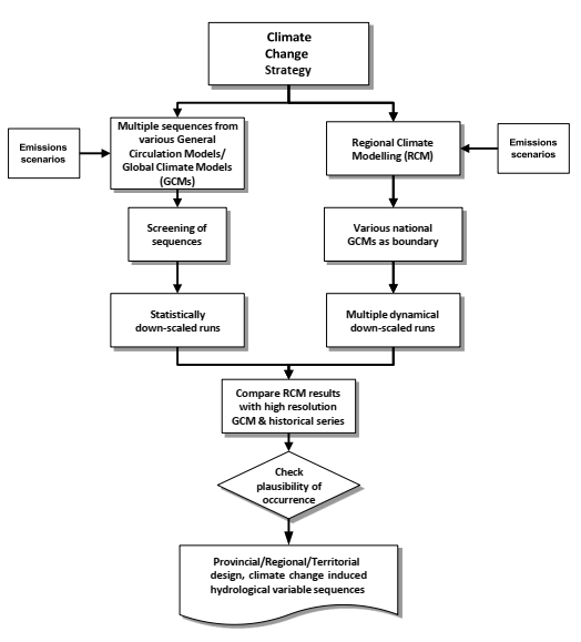
Figure 4.1 - Climate change application.
Text version - Figure 4.1
Flow chart identifies considerations to take into account when conduction flood hazard delineation.
A strategy for the application of climate change to flood hazard mapping will follow an ensemble approach requiring either statistical downscaling or a regional climate model approach using dynamic downscaling (see Section 4.1). Both approaches require the selection of emissions scenarios (Section 4.1.2). These may be selected on a most-likely approach or as setting upper and lower bounds to the flood hazard delineations. The downscaled ensembles or regional climate models are available for anywhere in Canada from CCCS, or directly from the originating agency. In many cases, future projected meteorological parameters are published for inclusion in verified hydrologic models, developed as described in Section 5.5 or in statistical regression analyses as described in Section 5.4.9. The qualified professional may start with these future meteorological parameters for the region of the study site.
Both approaches, whether using a model or regression analysis, require a comparison with the historical series and global climate change models to ensure the results are reasonable. The results are sequences of climate factors that will influence the streamflows arising from future climates.
Climate change practices are outlined in Table 4.1.
| Practices to Incorporate Climate Change into Flood Hazard Studies | |
|---|---|
| Step 1 | Select emissions scenarios from possible representative concentration pathways. |
| Step 2 | Select general circulation model for either statistical downscaling or regional climate approach. |
| Step 3a | Statistical downscaling approach: Screen the climate models, spatially disaggregate and compare with historical data to determine any bias correction needed to establish a weather generator of meteorological factors that impact extreme high streamflows and lake water levels. The weather generator components may be linked to future streamflows and water levels by linear regression. CCCS may develop some components of a weather generator downscaled when a need is justified for regional studies. |
| Step 3b | Regional climate approach: CCCs may be approached to produce some bias-adjusted water supply sequences from dynamically downscaled models available from its website. |
| Step 4 | Compare with the historical series and other global climate change models to ensure the results are reasonable as a check of the plausibility of occurrences. |
| Step 5 | Evaluate flood hazard delineation with the streamflows that result from the sequences of climate factors and a verified hydraulic model (see Section 6.0). |
| Step 6 | Consider a range of values from ensemble of results to quantify uncertainty. |
| Step 7 | Map the flood hazard delineation and report on the process following the requirements in Section 10.0. |
First, practitioners select which emissions scenarios (Section 4.1.2) will apply, depending on the greenhouse gas scenarios foreseen for the future. Next, they select the agency toolkit for use to generate the ensemble (Section 4.1.3) of future climate parameters that will reflect in streamflows and lake water levels from a range of emissions scenarios or a perturbation of input parameters. Alternatively, practitioners can select a series of models to generate ensembles of climate parameters and the resulting flows and levels. Sections 4.1.4 and 4.1.5 discuss the next step of dynamic or statistical downscaling and spatial disaggregation to map the model results to the study site. Once these model outputs are adjusted for bias, the meteorological values are compared to historical records; these are applied to the selected hydrologic model for producing climate change influence on the design flows.
When a regional flood frequency approach is available for the current design flows based on a regression analysis that included meteorological input, the factors changed due to the climate change models may now be used to generate new weather-based streamflows in the regression equations as future AEP projections.
4.1 Climate Change Information Data
4.1.1 Global Climate Models and General Circulation Models
The terms “global climate model” and “general circulation model”, both abbreviated to GCM, are generally used interchangeably to describe numerical models that represent coupled physical processes in the atmosphere, ocean, cryosphere, and land surface. Development of the most recent generation of GCMs has emphasized the representation of biogeochemical cycles, particularly explicit representation of the carbon cycle; hence, these global models are often referred to as Earth system models (ESMs). GCMs and ESMs are currently the most advanced tools employed to simulate the response of the global climate system to increasing greenhouse gas concentrations. They generally have a horizontal resolution of 100 to 250 km with typical internal timesteps of hours and periods of simulation that can reach thousands of years (Charron, 2014).
4.1.2 Emissions Scenarios
Projections of future climate change require projections of external drivers of change, such as greenhouse gas (GHG) and aerosol concentrations that are used as inputs to GCMs. With each new IPCC report, the terminology for pathways has changed. Pathways are standardized scenarios of radiative forcing and accompanying greenhouse gas, atmospheric aerosol, and land use change time series referred to as, for example, RCP2.6 (low radiative forcing pathway), RCP4.5 and RCP6.0 (moderate radiative forcing pathways), and RCP8.5 (high radiative forcing pathway). The higher the RCP, the greater the greenhouse gas and aerosol concentrations in Earth’s future atmosphere. Given current global GHG production, inclusion of RPC8.5 in any analysis would be prudent. With the new release of shared socioeconomic pathways (SSP) scenarios, these hydrologic and hydraulic guidelines will be updated in the next version of this document.
4.1.3 Ensembles
Like any other hydrometeorological models, GCMs are sophisticated but imperfect representations of reality and contain different assumptions about how to best represent complex physical processes, especially those that operate at spatial and temporal scales that are not explicitly resolved in the model. There are dozens of GCMs that have made projections of future climate, each with different assumptions and analytical methods. Due to the high level of uncertainty associated with using the water supplies from any one GCM, practitioners should use an ensemble of GCMs to project future climate variables. The Pacific Climate Impacts Consortium (PCIC, 2021) uses an ensemble of 12 different GCMs to conduct statistical downscaling for projecting future climate variables. Other scenarios are available in Canada (e.g., from the Canadian Centre for Climate Services, PCIC, Ouranos, etc.) and internationally (e.g., Coupled Model Inter-comparison Project [CMIP]). In addition, most providers have model ensembles driven by different GHG emissions scenarios (see Section 4.1.2).
4.1.4 Dynamical Downscaling by Regional Climate Models
Dynamical downscaling involves running a physically based climate model, referred to as a regional climate model (RCM), which operates at higher resolution, typically from 10 to 50 km, over a limited-area domain. Both past and future climate simulations in generating the RCM require that the RCM is driven at its lateral boundaries by output from a GCM. Because of the increased resolution, this approach captures more local variability in land cover, water surface area, topography, and other physical features, including local feedbacks, but the RCM will also inherit errors and biases that may be present in the GCM. In some cases, the results of dynamical downscaling may not provide any more useful information than the GCM. The benefits and costs (including potentially high computing power) of dynamical downscaling should be assessed at the initial stage of climate change assessment. Like GCMs, RCMs are developed at numerous institutions around the world, and most participate in the Coordinated Regional Climate Downscaling Experiment (CORDEX). CCCS has an inventory of dynamically downscaled RCMs for the various regions of Canada. These are continuously updated and as the resolution increases, the atmospheric feedbacks form the land-surface may be better represented. As an example, convection is not resolved in most RCMs, which can be problematic for extreme event analysis. Convective permitting schemes are slowly being developed for these next-generation models. It is important to be very specific about the version and source of the climate change models used in the study.
4.1.5 Statistical Downscaling and Bias Adjustment
Many bias adjustment methods exist, ranging from relatively simple “delta approaches” applied to bulk meteorological or hydrologic model outputs. Usually, the final GCMs and RCMs outputs are corrected for systematic biases at basin scales. Consequently, flood-relevant GCM and RCM data typically require some post-processing like many similar efforts to produce reliable estimations. Further downscaling of GCM or RCM outputs to higher spatial resolution may also be required, in which case statistical downscaling methods can be applied either separately or in combination with bias corrections.
Statistical downscaling involves the combination of climate model projections and local or regional observations to provide climate information with more spatial detail. Different approaches can be used, including regressions, stochastic weather generators, and machine- learning algorithms. In addition to helping with resolution, downscaling allows the derivation of the other variables needed for flood mapping.
The Pacific Climate Impacts Consortium (PCIC, 2021) has produced a publicly available, statistically downscaled ensemble of GCMs to an approximate grid size of 10 km. A number of publicly available statistical downscaling tools exist (e.g., Wilby et al., 2002, Hessami et al., 2008). This approach is generally quicker and requires less computing power than dynamical downscaling. However, it does not attempt to reproduce atmospheric physical processes, instead relying on statistical relationships between climate model outputs and local or regional observations. Statistical downscaling approaches (e.g., regression-based methods) assume stationarity of statistical relationships, as well as credible simulation of larger-scale variability by the climate model.
Although statistical downscaling provides more spatial detail, it is not certain for many locations whether the results of downscaling will be more accurate than using data at the resolution of the climate models. The initial stage of a climate change assessment should weigh the benefits and costs of statistical downscaling. More step-by-step methods are being evaluated and will be part of the next version of this document.
4.2 Studies in the Canadian and Global Context
The Federal Flood Mapping Guidelines Series document, Case Studies on Climate Change in Floodplain Mapping (NRCan, 2018), provides three examples where climate change impacts were assessed for flood hazard studies. Additional case study examples are planned for future versions of this document.
Other examples of the application of climate change projections to Canadian watersheds are provided in Khaliq (2019), Rajulapati et al. (2020), and Zaerpour et al. (2021). A recent article (Wasko et al., 2021) provides the practical approaches to the incorporation of climate change in flood flow assessments from a global perspective.
4.3 Sea-Level Change Projections
Projections for sea-level change may be required to be incorporated into riverine flood delineation studies. The general procedure involves reviewing guidance from NRCan (James et al., 2021) on site-specific relative sea-level change, and selecting scenarios and planning horizons based on acceptable risk and design life (e.g., Lemmen et al., 2016). The relative sea- level change projections are then used as downstream boundary conditions for the riverine (hydraulic) modelling. When a given flood probability is estimated over a long period into the future, practitioners may use cumulative probabilistic techniques to account for collective flood probabilities due to increasing sea level.
Relative sea level (RSL) refers to the relative sea-level change that is experienced on the coastline and is a combination of global sea-level rise and vertical land motion. Flood hazard analyses and mapping that accounts for RSL should use up-to-date scenarios from national scientific reports (e.g., James et al., 2021; Lemmen et al., 2016; Han et al., 2016). Land uplift contributes to relative sea-level fall, while land subsidence adds to relative sea-level rise. In Canada, a dominant source of vertical land motion is the delayed response of the solid earth to the weight of the ice sheets, a process called glacial isostatic adjustment or postglacial rebound. Although this process is resulting in land uplift across much of mainland Canada, it is causing land subsidence in many coastal regions. NRCan regularly updates projected RSL changes (e.g., James et al., 2021).
4.4 Summary of Strategies for Consideration of Climate Change
In summary, the first step is to decide which emissions scenario(s) and time horizon(s) to consider for a flood hazard delineation under future climates. The jurisdiction may dictate the decision. Secondly, either a set of downscaled ensembles or an ensemble of regional models will determine the factors that influence the future meteorological parameters for the design flow assessment. Practitioners may assess the changes in the future flow assessment from the mean and range of the ensemble predictions. A thorough review by qualified reviewers not involved in the project should precede the publication of the design flow assessment report covering the climate change analyses, as outlined in Section 10.0.
5.0 Procedures to Assess Design Flood Events
A description of the assessment of the design or regulatory flood events, the hydrologic procedures, and supporting flood hazard delineation is included in this section. These procedures may include both peak flow estimates and design flood volumes if the stream empties into a small lake where levels depend on the flow volumes. Design flow and water level events are usually expressed in terms of a return period or an annual exceedance probability (AEP). For example, a flow event with a 1% AEP and a flow event with a return period of 100 years are equivalent. As noted in Section 1.4, the concept of return periods can be misleading to a non-technical audience. Therefore, this document uses the term “AEP” instead of “return period”. In some jurisdictions, a historical extreme meteorological event is used to define the design flow event. These procedures recommend that provinces and territories set a design or regulatory flow to at least the equivalent of a flow of a 1% AEP.
Table 5.1 explains the hydrologic procedures that are necessary to develop reliable and realistic design flows. These are cross-referenced in tabular form and illustrated in Figure 5.1.
| Hydrologic Practices | |
| Step 1 | Define hydrologic outcome according to the design flood event criteria of the jurisdiction (Section 5.1). |
|---|---|
| Step 2 | Gather data (Section 5.2): Identify all sources of relevant data and historical information in the defined hydrologic region. Include hydrologic and meteorological data that meet key data requirements. Document sources of historical information and data selected. Use the maximum flood record available. |
| Step 3 | Investigate non-stationarities and homogeneity (Section 5.2): Conduct a quality assurance and quality control check of the hydrologic data including verification of stationarity and homogeneity. Identify the effects of flow regulation and diversion on hydrologic data to ensure it is appropriately addressed by the selected hydrologic procedure. |
| Step 4 | Select analytical approach (Section 5.3). |
| Step 5 | Conduct a flood frequency analysis (FFA) (Section 5.4): Conducting a single station FFA if historical information and systematically collected flow data are available. Practitioners must be aware of the uncertainties of this approach and confirm that the data meets the underlying assumptions. When sufficient data are not available to support a single station FFA, conduct a regional FFA (RFFA) for a hydrologically homogeneous region having a sufficient number of streamflow records and adequate periods of record. |
| Step 6 | Conduct a deterministic hydrologic analysis (Section 5.5): This is the preferred approach when design flows are based on a historical storm or synthetic design storm, a flood hydrograph is required, or where the watershed has experienced land use changes. |
| Step 7 | Incorporate the impact on design flood events of future non-stationarity caused by factors such as climate change, alternate land uses, regulation, and morphological changes. Details regarding the assessment and consideration of climate change are provided in Section 4.0. |
Step 8 |
Determine the design flood flows or water levels. Continuous simulation deterministic models are used where long-term meteorological data is available to generate long-term discharge series. FFA methods can be applied to historical records or to the output of hydrologic models to calculate design flows for specific AEPs. Single event deterministic hydrologic models are used for regions that require historical storms or synthetic design storms or in cases where there is insufficient data to support continuous simulation modelling. FFA on water levels can determine water levels of specific AEPs. |
Step 9 |
Evaluate results against the design flood event criteria of Step 1. Verify and document study results. Whenever possible, verify results of a chosen hydrologic procedure (FFA, RFFA, or hydrologic modelling) by comparing results with one or more alternative procedures. Maximum floods known from paleontological, historical, or Indigenous knowledge outside the systematically observed records may provide context for the results, considering varying conditions. Qualified reviewers not involved in the project may assess the data, methods, and outputs of the analysis. |
Step 10 |
Document all aspects of the selection, implementation, testing, verification, results, sensitivity, repeatability, and uncertainty associated with the selected procedure. Include how the community was engaged in the study and its results. Refer to Section 10.0 for an overview of reporting requirements. |
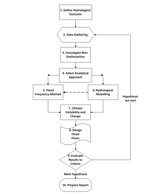
Figure 5.1 - Hydrologic procedures.
Text version - Figure 5.1
Flow chart showing the hydrologic procedures of a hydrologic outcome.
5.1 Definition of Hydrologic Outcome
The first step in any hydrologic procedure is to define the outcome at the location of the study site. For a flood hazard delineation of a particular watershed, the outcome will be defined by the relevant jurisdiction. It may be a flow (or water level) corresponding to a specific AEP (e.g., 1%, 0.5%), flood events corresponding to a number of AEPs (e.g., 5%, 1%, 0.5%), or a flow generated by a historic extreme meteorological event. The outcome should incorporate impacts of climate change and known future land uses. The hydrologic outcome or design flood event, as shown in Figure 2.2 of Section 2.0, will be used in the hydraulic model to determine the extent and depth for the flood hazard delineation. The definition of a flood fringe may require the determination of velocities throughout the extent.
| Provinces and Territories | Design Flood AEP | Historical Design Storm Event | Freeboard |
|---|---|---|---|
| Alberta | 1% | - | - |
| British Columbia | 0.5% | - | - |
| Manitoba | 0.5% | - | - |
| New Brunswick | 1% | - | - |
| Newfoundland and Labrador | 1% | - | - |
| Nova Scotia | 1% | - | - |
| Northwest Territories | - | - | - |
| Nunavut | - | - | - |
| Ontario | 1% | Hurricane Hazel storm (1954) Timmins storm (1961) |
- |
| Prince Edward Island | 1% | - | 0.65 m |
| Québec | 1% | - | - |
| Saskatchewan | 0.2% | - | 0.5 m |
| Yukon | - | - | - |
The selection of appropriate procedures depends upon the type of hydrologic “problem” under study and the availability of data required to solve it. For example, in some jurisdictions specific or several different design floods require assessment (e.g., 5% AEP, 1% AEP, 0.5 % AEP, etc.). If sufficient flow data is available, procedures such as a single-station FFA or an RFFA may achieve the determination of design flood events of a specific AEP. The analyses of design floods based on water levels, such as ice-related flooding and lakeshore flooding, may also rely on FFA procedures. However, other jurisdictions define the design flood event by the transposition of a historical storm event over the watershed of the study site. In these cases, hydrologic simulation models are used. Also, significant land use changes indicated by known future land use plans upstream of the study site require a hydrologic model to simulate the future conditions.
5.2 Data Requirements
Design flow assessments require the precise gauge location, water level or hydrometric records, and regional hydrologic information, like RFFA or storm transposition data, as a minimum. If hydrologic modelling is required, it will also require meteorological forcing information and the relevant geospatial data.
5.2.1 Data Preparation and Gap Filling
The recorded streamflow or water level at a gauge is considered the best estimate of all hydrologic methods. This stems from the understanding that the recorded data is the integrator of all hydrologic processes in the watershed. Therefore, the best approach to compute design events for frequency-based estimates ensures that the data series are obtained with due thoroughness. There are two basic scenarios for the way recorded data are used, one if the mapping project or the location where the design flows are desired coincides with the gauge location, and two, where the information is needed away from the gauge location. There are times when the recorded elevations or flows are unavailable or not reliable due to floods, for example, when the gauging stations are destroyed in the flood event. Flows determined to the full length of a usable record should then be used with peak values obtained by indirect means.
Figure 5.2 captures the different pathways and steps in reconstructing the missing data and extending records from reference and neighbouring hydrologically similar watersheds and regional basins. It should be noted the regional approaches described here are for daily flow. The data series generated in these steps provide the basis for all flood frequency analysis. The procedures for regional analysis of flood estimates are captured later in Section 5.5. As presented in Figure 5.2 there are five potential pathways, labelled as A to E in the boxes with uncertainty increasing from Steps A to E. These are briefly described below.
- If the dataset is free from regulation and with full record, it can be directly used for further testing to ensure its usability through the statistical parametric and non- parametric tests for establishing the design flow.
- When the time series is influenced by the presence a water regulation structure, the naturalized series is computed through any of the reverse routing methods. These may include adjustments for diversions and additions and for daily evaporation if the lake or reservoir is in an area of net evaporation (Section 5.2.7).
- If the series is partial with a reference station available for use to extend the data, the suggested approach is the Maintenance of Variance Extension (MOVE.1) or an equivalent technique.
- If the series is partial with no reference station available, the suggested approach is the flow duration curve method (Hughes & Smakhtin, 1996).
- At the point of interest, if there is no data available, a regional drainage area method is suggested. In such cases, the synthesized data need to be verified by other approaches (Section 5.2.3).
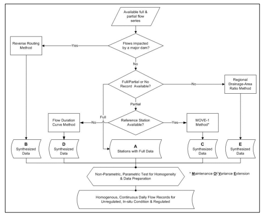
Figure 5.2 - Procedure for preparing flows for analysis.
Text version - Figure 5.2
Flow chart describing the procedure for preparing flows for analysis.
5.2.2 Extension of On-Site Instantaneous Flow Records
In many cases, jurisdictions may require the use of annual maximum instantaneous peak flow (QP) data when undertaking hydrologic procedures, such as single-station FFA. Often, the length of record for QP at a gauge is less than the period of record for annual maximum daily peak flows (QD). In these cases, the QD data record may be used to extend the QP dataset.
There are several approaches to compute peak instantaneous discharge when the maximum daily flows are available.
- Using the period of record when the two types of data overlap, the following relationship may be developed in which “a” and “b” are variables describing the relationship between QP and QD:
QP = a · QDb - Fuller’s method (Fuller, 1914) could similarly be applied to compute the peak instantaneous discharge values. In this case the drainage area “A” of the basin was found to be important: the larger the drainage area, the smaller the peaking factor, and vice versa for smaller basins. In a generic form, the variables “c” and “d” are estimated from regional analysis:
QP = QD · ( 1.0 + c · A-d )
- The 3-day method is a more data-dependent technique developed by Sangal (Sangal, 1981) and applied to over 560 basins in Ontario by Moin and Shaw (1985). This method is based on a triangular hydrograph and the following formula where the variables are the mean daily flow of three consecutive days, designated as QD1 on the day before, QD2 on the day of maximum daily discharge and QD3 the day after.
When α = 0
- Fill and Steiner (2003) developed regional equations based on Sangal’s approach for watersheds in Brazil. The formulation took the following form:
Similar relationships could be developed for other regions based on the information available. - Several newer techniques have been available using artificial neural networks (ANNs) and adaptive neuro-fuzzy inference systems (ANFISs) (Nayak et al., 2004).
In all these methods, care should be taken to consider the size of the basins when such equations are developed. These ranges should be respected. The result can subsequently be applied to the period when only annual maximum daily peak flows exist to estimate the equivalent instantaneous peak flows. Of course, the application of such procedures is applied to the two series of data when both peaks are from the same event.
5.2.3 Transposition from the Hydrologically Similar Watersheds
This section describes the pathways briefly highlighted in pathways C and E. The most common method of extending or infilling missing streamflow records for a study stream is achieved by transposing flow records from a gauge of similar hydrologic characteristics with a longer period of record than the study stream within the study watershed or from a nearby gauged watershed. If the periods of record overlap, a site-specific cross-correlation model can be derived and applied (pathway C). If not, a more generic, possibly physiographic, relationship can be employed (e.g., one based upon the ratio of drainage areas to a power equal or less than 1, depending on regional characteristics [pathway E]). A classic approach is presented in the recent work carried out in the Souris Hydrology reconstruction (USACE, 2019).
5.2.4 Pre-Record Floods (Historical Information)
Uncertainty in hydrologic flood frequency analysis can be reduced by inclusion of historical floods that occurred prior to the systematic collection of hydrometric records (pre-record floods) and may not be captured in the dataset. These floods may have associated physical, photographic, or other evidence useful to estimate flood magnitude. The historically observed water levels (e.g., available from flood markers) can be used to derive flow and applied in hydrologic procedures. The usefulness and accuracy of the derived flow information will depend upon the reliability of the stage-discharge relationship at the observation location, or the inclusion of a detailed hydraulic model. For extreme floods, the stage-discharge relationship may have to be extended empirically, leading to considerable uncertainty in the flow estimate. The benefits of including such estimates must be balanced against the uncertainty.
Evidence of historical and pre-record floods can be found in newspapers, municipal records, universities, libraries, historical photographs, Indigenous knowledge, and other sources. Using pre-record floods in an FFA may reduce the uncertainty associated with high-magnitude flood events and may better align the dataset with the local experience of the community affected by those flood events.
Historical data should be validated to the extent possible and ideally corroborated from multiple sources (e.g., newspaper article description of inundated areas matching a photograph with identifiable landmarks).
Consideration of “perception levels” is important in evaluating pre-record floods. Research should be conducted to determine the minimum threshold flood event that was recorded by people who experienced the flood. Guidance on perception thresholds is included in USGS (2019), Gerard and Karpuk (1979), and Associate Committee on Hydrology (1989).
5.2.5 Paleo Records
It is possible to gather information on floods that occurred prior to the collection of historical records through the collection of physical, geomorphological, dendrochronological, and other data.
Paleofloods are flooding events, including those that occurred several thousand years ago, that occurred prior to the collection of hydrologic records. Geographical and physical evidence of paleofloods includes rock alcoves with sequences of slackwater deposits, scarring on trees, gravel bar deposits, erosional scars, and excavated soil (Jarrett & England, 2002). Specific expertise in geomorphology, geology, or a related science is required to identify and date these features. In addition to the identification of paleoflood events, it is possible to identify an absence of paleoflood events, which increases the confidence level in the existing hydrometric dataset (i.e., a reasonable degree of confidence is gained that the hydrometric record does not erroneously omit significant flood events).
Botanical information is also useful to “extend” streamflow records by examining deposited sediments around tree trunks, examining tree ring patterns, and other methods. Specific expertise is required for these types of analyses.
The direct inclusion of flow estimates based on paleofloods in a hydrologic dataset used for frequency analysis should be used with extreme caution. Qualitative checking of results is warranted when using such data, as well as when performing a more conventional flood frequency analysis. In many areas, the impact of glacial isostatic rebound needs to be considered and accounted for in the analysis.
5.2.6 Assessment of Streamflow Regulation
There are over 900 major dams in Canada and thousands of small dams. Most large dams in Canada are used for hydroelectric power generation, though other uses include water supply, irrigation, flood control, and recreation. Streamflow regulation alters the shape of the streamflow hydrograph, including timing and shape of peaks. This may result in historical records of downstream flows being non-homogeneous (pre- versus post-dam construction or partly or wholly uncorrelated changes to natural environmental driving flood mechanisms with the regulation policy over time), which should be considered when undertaking an FFA or RFFA analysis (Section 5.4). One possible technique is deregulation of the data, in which reverse routing is used to estimate “natural” inflows upstream of the regulation. In addition, if regulation is by means of a fixed structure with little storage compared to the flood volume, it may be possible to consider the annual maximum data to be uninfluenced by the regulation.
Methods for assessing the impacts of regulation on small watersheds have been proposed (e.g. Moin and Shaw (1985, 1986), López and Francés (2013)). The appropriateness of these, or other methods vary substantially based on the region, the flood generating processes, and the scale of the watershed. The most appropriate method for dealing with regulation should be assessed by a qualified professional.
5.2.7 Method to Naturalize Regulated Flows
The intent of naturalizing the flow, as noted in Figure 5.2, is to obtain what the streamflow values would have been had the dam not stored the flow causing attenuation of the peak and extra evaporation nor had any diversions redirected the flow into or away from the stream for various purposes. Figure 5.3 shows how to naturalize recorded flows when considerable storage, diversion, or evaporation has occurred upstream of the point of interest. Practitioners will need the inputs as shown on Figure 5.3 to follow the calculation steps mentioned below.
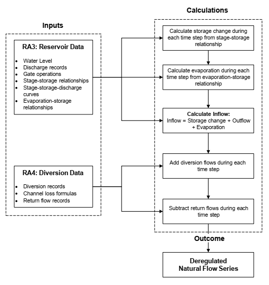
Figure 5.3 - Naturalization of regulated flows.
Text version - Figure 5.3
Flow chart shows how to naturalize recorded flows when considerable storage, diversion, or evaporation has occurred upstream of the point of interest.
The inputs required to obtain the natural flow where a reservoir has interrupted the flow are the following:
- Water level and discharge records of the dam, either as directly measured or as derived by gate operation records or from the stage-storage-discharge curves to determine the outflow.
- Records of any flows diverted, either into or out of the reservoir.
- Stage-surface-area-storage relationships to calculate the surface area and storage volumes from changes in water levels.
- Evaporation-surface-area relationships, where the reservoir is in an area of net evaporation, that is, low precipitation. Care should be taken to respect measurement units for evaporation, usually in mm, and reservoir area, typically in km2 or ha. The evaporation and precipitation records from nearby meteorological sites may be applied, or where evaporation is unavailable, standard evaporation formulas based on temperature and wind records can be used. Consideration of evaporation is usually only required in areas of net evaporation, such as the Prairies and the interior of British Columbia.
Practitioners may then use this data to calculate the natural inflow to the reservoir and what would have flowed had no attenuation nor had any significant evaporation occurred. For the comparison of hydrologic models determining high flows or for FFA, use a small time-step no longer than a day:
- Calculate the flow into the reservoirs from the increase in water level of the reservoir and the discharge, using the stage-storage- discharge relationships or discharge records.
- Add the flows diverted out.
- Subtract the flows returning in.
- Add any water evaporated, as calculated from the storage relationships during the inflow calculations, where applicable.
Streamflow diversion involves moving water out of streams and is much less common than dam regulation in Canada. However, any diversions in the modelled stream and in the study area should be identified and data on diverted water obtained, including operating procedures. The inputs required are the measured diversion records for irrigation or other consumptive uses, and records of any return flows. When water is diverted out of a reservoir or stream, the flow is added and return flows are subtracted.
If the diversion records are at the point of diversion, upstream of any channel losses, no allowances for seepage or evaporation are required. Otherwise, estimates of water lost to channel seepage and evaporation between the point of diversion and the point of measurement need to be added to the records of the water diverted. Again, use a small time-step of a day or less for high-flow studies.
Modelling can be applied to understand both unregulated and regulated streams. If operating procedures are clearly defined and quantifiable, they can be applied directly into hydrologic models. Caution is required in deregulating the flow in presence of wind-induced water level changes that may lead to errors and potential negative flows. Therefore, where wind-related impacts are prevalent, the reverse routing method for the deregulation of flows induces a large amount of uncertainty. It may be better to restrict this evaluation to the duration around flood events.
5.2.8 Flow Data Quality Analysis
The final step after collecting and synthesizing the data is to perform a quality control review. Practitioners should subject the data to visual analysis and statistical tests to assess the homogeneity of the resulting unregulated, continuous daily flow records for the gauges having periods of regulated data. The flow data may be tested for non-stationarity before deciding on the approach to use to assess the design flow.
5.3 Selection of Analytical Approach
Two types of hydrologic approaches are used to determine design events. The first approach uses measured streamflow data to perform a single-station FFA or multiple-station RFFA and is appropriate when sufficient and reliable hydrometric records are available. The second approach, hydrologic modelling, simulates the watershed response to either a continuous sequence of meteorological events or a single design rainfall event. These generate either a synthetic flow series that can be used to perform a single-station FFA or a single time-varying hydrograph of flows for the design event. Hydrologic modelling is used for analyzing climate change impacts when significant changes to the land use upstream of the study site are planned (e.g., future development, etc.) or have changed since the historical streamflow data were recorded.
Often practitioners may start with the first approach to assess the design flow or water level, however, finding insufficient data, non-stationarity in the recorded streamflow or water level data, or recognizing significant planned future land use changes, the professional may require an alternative method and extra analysis will be necessary.
In any case, multiple procedures should validate results from any “preferred” procedure. Rigorous evaluation and comparison of the results and historical observations, compounded with experienced professional judgment should evaluate the results. Finally, any hydrologic analysis must be documented and repeatable, with all assumptions clearly stated, including software, model, and versions.
5.4 Flood Frequency Analysis Approach
Flood frequency analyses use the statistical properties of observed, historical, or derived flow or water level records to define a relationship between flow magnitude (or water level) and AEP at a given site. The relationship is used to estimate the flow (or water level) for one or more desired flood frequencies. This section describes the techniques of the process (see also Khaliq, 2017).
Figure 5.4 shows the different procedures that occur under an FFA method, either for a single station or RFFA.
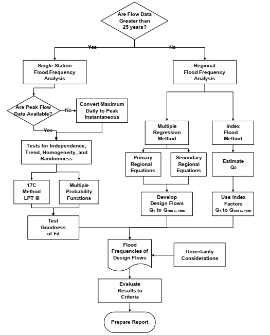
Figure 5.4 - Procedure for flood frequency analyses
Text version - Figure 5.4
Flow chart showing the different procedures that occur under an FFA method, either for a single station or RFFA.
When undertaking a single-station analysis, practitioners will analyze the flood frequency for either the recorded or synthetic peak instantaneous flows. Synthetic peak flows are estimated from the annual maximum (AM) mean daily flow using regression equations or other methods as explained in Section 5.2.2. Practitioners will determine which distribution better describes the flow data, a USGS 17C Log-Pearson Type III statistical distribution (see e.g., USGS, 2019) or one from multiple probability functions as described in detail later in this section. As part of this process, practitioners may assess the degree of influence of zero flows or potentially influential low flows that may be adversely affecting the distribution’s fit in the area of most interest—the largest floods. In case of zero flows or upon identification and for treatment of zeros and potentially influential low flows in the FFA, and until proper software with multiple distributions is developed, it is recommended that the methods described in USGS Bulletin 17C (USGS, 2019) be employed. After determining the goodness-of-fit of the selected distribution, they will determine the probabilities of flows. The fitting of probability functions to streamflow series is called an FFA and is described in Sections 5.4.1 to 5.4.7.
When undergoing an RFFA, practitioners will analyze the flood frequency by either a multiple regression method or by an index flood method (Moin & Shaw, 1985, 1986). A multiple regression method explores the strength of correlations between a number of potential causal terrain and meteorological factors in a hydrologic region and a series of AEP flood peaks. This results in primary regional equations of higher predictive strength and secondary regional equations that further refine the predicted flows for the recorded flows at similar stations in the region (see Section 5.4.8). From these equations, applied to the watershed characteristics and meteorological factors of the study stream, practitioners derive the design flows for various annual exceedance probabilities.
An index flood method uses an analysis of hydrologically similar stations in a region to determine the index factors that relate the mean annual flow to the various percent AEP peak flows. At the study stream, practitioners determine the mean annual flow (see Section 5.4.11) and applies the index factors for the region to determine the design flows for various annual exceedance probabilities.
Once the design flows are determined and verified, practitioners can incorporate climate changes (Section 4.0) and describe uncertainties (Section 9.0). Qualified reviewers not involved in the project should examine the analyses before the final report (Section 10.0) presents the design flow according to the criteria for the flood hazard delineation of the jurisdiction.
Floods of interest for flood hazard delineation, such as the 1% AEP, are often much greater than any flood recorded in the relatively short period covered by systematic records in Canada. Extrapolating a simple statistical model of limited record length of a complex physical process introduces uncertainty in estimating design floods. In such situations, regional flood frequency analysis procedures are advocated to complement the single-station FFA. This also includes incorporating adjustments to the single station skew and combining independent estimates of design flows to improve the derivation of the flood quantile and reduce its uncertainty (USGS, 2019).
While this discussion focuses on conventional peak streamflow flood frequency analysis, many of the concepts are equally applicable to flood-duration-frequency analyses (e.g., Cunderlik et al., 2007) and to analyses of flood volumes, water levels, seasonal peak flows, and other natural phenomena, including rainfall.
5.4.1 Key Assumptions of Flood Frequency Analysis Approach
Use of FFA assumes that the record of observed floods can be treated as independent random variables drawn from a homogeneous and representative population that remains unchanged over time. A variety of statistical tests exist to help practitioners determine how well a peak flow record meets each of these pre-requisite assumptions for FFA. Greater departure from these assumptions requires increased caution and explanation of the causes when evaluating results and increases the importance of independent checks. In some cases, it is possible to improve the suitability of the FFA by undertaking additional data analysis. In other cases, the consultation and input of specialists in related fields may be required.
5.4.2 Record Length
Extrapolation contributes significantly to the uncertainty of the FFA’s results. The most effective way to mitigate this uncertainty is by maximizing the record length and representativeness of the available data record. Approaches commonly taken to do so transition from a single-station analysis, to one that includes adjustments to parameters or moments based on regional information, to combining an independent estimate of the flood quantile. Supporting this process is quantification of the uncertainty of the estimates.
While a number of suggested “rules of thumb” exist based on some dated and some newer methods, these resolve in extending the information. Practitioners use different thresholds for moving from a single station to using regional information as captured in the following. Single- site FFAs should only be conducted in cases where the period of record is greater than 10 years (England et al., 2017). However, obtaining reliable results from a single-station FFA requires a period of record that significantly exceeds the AEP of interest (e.g., Klemeš, 1987). This is impractical in the Canadian context given the relatively short record lengths at most single stations. The traditional approach taken has been to obtain an estimate based on a “reasonable” record length proportional to the desired AEP.
For example, in the Canada-Ontario FDRP, an extensive regional analysis suggested a procedure captured in Figure 2.5. The suggested cut-off was a record length less than 25 years. In other regions, this threshold could be adjusted based on available data. A common rule has been to avoid extrapolating to AEPs more than double the length of the available record (e.g., limiting extrapolation from a 50-year record to the 1% AEP flood, which is equivalent to a 100- year return period). Some references have provided specific recommendations; for example, Coulson (1991) proposed specific minimum record lengths for estimating various AEP flood events in British Columbia.
These minimum criteria could be insufficient if the period of record happens to correspond to a period of unusually high or low flood activity. Records of a short period require validation by consulting historical sources of information or data from hydrometric stations with similar hydrologic conditions and with longer records. Sections 5.2.2 to 5.2.5 describe approaches for extending the period of analysis by transposing data from other hydrologically similar gauges, and incorporating floods and historical streamflow, botanical, and paleo information that pre- date the systematic record.
Upon compiling the record, it is necessary to determine whether the analysis will be based on instantaneous or daily average peak flow data. If the record incorporates winter floods, including ice-jam-related events, practitioners must also determine whether the analysis will consider calendar years or hydrologic years. These considerations may affect the amount of data available.
5.4.3 Data Quality and Completeness
Peak flow data is usually subject to high uncertainty. Because FFA is sensitive to a small number of high and low streamflow observations, care is needed to understand the uncertainties that are implicit in the measurement process. Additionally, data missing from broken and incomplete records should be filled in wherever possible.
Once screened and reviewed for quality, practitioners should plot and review the record to determine its likelihood to produce a satisfactory FFA. Outliers, step-changes, slope breaks, and when floods occurred could indicate that different flood-generating processes may be present.
Low outliers that could influence the FFA (e.g., zero-flow years and potentially influential low flows) should be screened and removed using a statistical test, such as the multiple Grubbs- Beck test (Cohn et al., 2013; England et al., 2017). Procedures outlined in Bulletin 17C (USGS, 2019) may be followed for addressing such situations. Once removed, their occurrence must still be reflected in the overall analysis.
Extraordinary floods (high outliers) may be identified using a similar process but are usually retained due to the importance of high flows for design flood prediction. High outliers may be the result of a different flood-generating process, requiring a more complex analysis as discussed in the next section (5.4.4). As well, observed historical information, when known, should be incorporated into the analysis, noting that the inclusion of such information would also be reflected in the plotting position.
The policy implications of regulation and inter-basin diversions must be accounted for, since FFA should be applied to a “naturalized” peak flow series. Section 5.2.6 discusses how to handle regulated flow records. Practitioners must determine whether it is appropriate to re- regulate the resulting peak flow based on anticipated operating procedures and stakeholder risk tolerances.
5.4.4 Analysis Structure
For a single-station FFA, there are three key criteria to consider in terms of analysis structure (each is described below in this section):
- Annual maximum (AM) versus peaks over threshold (POT).
- Combined population versus single population.
- Whether the analysis must account for non-stationarity.
The term AM refers to the creation of a historical flood series that includes only the highest peak flow in each year. This method is appropriate when the largest annual flows occur during the spring freshet. In such cases, there may only be one or possibly two independent peak flows occurring in a given year. For locations (e.g., urbanized catchments, areas with little snowpack, etc.) that experience high flows during different seasons or from different causative factors (e.g., snowmelt, rain on snow, different types of systems causing rainfall), an AM approach may not capture important information about flood genesis and behaviour, particularly for shorter record lengths. For example, some years might have multiple independent large floods while other years lack even a single significant event. To address this, all peaks above a selected threshold are included in a POT analysis, also referred to as a “partial duration series” analysis. POT analyses are more complex than AM analyses, and identification of an appropriate threshold may be complicated. POT results are asymptotically comparable to AM results for lower AEPs (e.g., 1%). However, there can be large differences for higher AEPs (e.g., 50%, 20%, 10%) (Bezak et. al., 2014). As well, POT analyses may result in lower sampling variance of the design flow events than those provided by AMS analyses for AEP < 0.10 when the POT series contains a sample size of greater than or equal to 1.65N, with N being the number of years of systematic data collection (Cunnane, 1973).
In general, a time series of annual peak-flow estimates may be considered to be a random sample of independent, identically distributed random variables. The peak-flow time series is assumed to be a representative sample of the population of future floods. This assumption is contingent upon conducting exploratory data analysis and further physical knowledge of the system. In essence, the stochastic process that generates floods is [also] assumed to be stationary or invariant in time. (USGS, 2019).
The exploratory data analyses and knowledge of the physical properties that are resulting in flooding underpin how to proceed with an FFA and with the selection of approaches for conducting an FFA. As well, there may be evidence that different flood-generating mechanisms are causing problems in single-density functions fitting the annual maximum series. This may be visible when viewing the frequency plot and could be in the form of “dog-legged” curves, where the most extreme observed floods depart from the theoretical frequency distribution.
Most FFAs have tended to be based on a “single-population” analysis of AM where the sample of observations is assumed to be drawn from a stationary, or assumed stationary, and homogeneous process. In some cases, knowledge of the physical properties of the mechanisms generating flooding may indicate that there may be two or more different (potentially also stationary) processes that contribute to the magnitude of the flood event, such as ice jams, snowmelt, and rainfall resulting from different causative meteorological events (e.g., hurricanes, stationary cold lows, mesocyclones).
When there is evidence that the AM series is not drawn from a homogenous (single) population and that to proceed with a traditional FFA may result in an inability to accurately depict the frequency-magnitude relationship, practitioners may explore the use of more complex frequency models. One approach is to adopt the use of a model that allows the separation of high versus low floods in the fitting of the parameters of the frequency curve to the AM series, such as the Wakeby distribution. This is done under the realization that different causative factors are at play and are compounding the analysis, and there may not be adequate information and data to support a “combined” frequency analysis.
In theory… an argument exists for treating most Canadian series as composed of two or more samples from different populations. Practically, however, such treatment considerably complicates the preparation of a frequency analysis, and there is little reason to do so unless treatment as a single population produces a peculiar shape of frequency curve or there are reasons for determining separate design floods of the two [or more] types. (Associate Committee on Hydrology, 1989)
When conditions warrant its use, a combined-population analysis is advisable. A combined- population analysis, also classified as a compound impact event, creates a separate FFA for each process and combines the results into a single composite magnitude-frequency or stage- frequency relationship. As mentioned, a combined-population analysis is more complex than a single-population analysis. The more complex approach is usually only considered for situations in which:
- There are distinct mechanisms evident in the historical record (i.e., observed peak flows show evidence of two or more population sources) and there is an indication that these differences will significantly influence the estimate of the design flow estimates at the desired AEP.
- There is a need to capture the implications of climate change or land use change for each of the different, dominant flood mechanisms and their populations.
- There is sufficient information and data available for each of the dominant flood- generating mechanisms to support a combined frequency analysis.
Stationarity, or that the variable is invariant in time, is assumed in most FFA projects using traditional tools. However, more recent FFA tools provide the option of accounting for non- stationarity (e.g., El Adlouni et al., 2007; Razmi et al., 2017). These newer non-stationary FFA tools are more complex than traditional FFA tools. Practitioners must determine whether the additional complexity is required. For example, it may be more cost-effective to account for climate change by applying regional factors established by climate change analysis (Section 4.0) to the results of a stationary FFA.
5.4.5 Software Packages
While a variety of software packages are available for conducting single-station FFAs, these guidelines include only four, with a full makeover required in one case. Listed in no particular order are ECCC’s Consolidated Frequency Analysis (Pilon & Harvey, 1993), HEC-SSP (USACE, 2019), and Floodnet RFA (NSERC, 2020). HyFran (El Adlouni & Bobée, 2015) is a commercial product that performs multiple distributions while fitting the data by several methods.
Most software packages offer a choice between multiple probability distributions, though not all programs offer the same options. Specific software packages for FFAs should be chosen based on considerations of input data, computational methods, outputs, and the application of results. It is important to document the reasons for model selection. A review of selected FFA software tools is available in Khaliq (2017).
5.4.6 Probability Distributions
Some probability distributions are well suited for FFAs based on theoretical criteria. For example, the Extreme Value Type I (commonly known as Gumbel) distribution has a strong theoretical basis for AM applications, while the related Generalized Pareto distribution is preferred for POT analyses. In other cases, an “institutional” distribution is adopted to define a common standard of practice. Through the US Geological Survey Bulletin 17C (England et al., 2017), the US adopted the Log-Pearson Type III distribution as an institutional distribution. In Canada, many FFA studies consider at least one distribution drawn from each of the normal, generalized extreme value, and Pearson distribution families. Other distributions with more parameters (e.g., the five-parameter Wakeby distribution) are better suited for analyses where a combined frequency analysis may be warranted, but there may be insufficient data available to support such an analysis. However, practitioners must use their judgment in assessing the performance and justification of the selection of a particular distribution for their investigations.
Once a distribution has been selected, it must be “fitted” to the observed flood data. The ease, variety, and objective nature of mathematical curve fitting has relegated the once-popular method of graphical fitting to rare extenuating circumstances.
There are numerous mathematical methods for fitting distribution parameters, including least squares, method of moments, probability-weighted moments and L-moments, and maximum likelihood and generalized maximum likelihood methods. Some parameter-fitting methods are better suited to particular distributions than others are. More specialized statistical approaches like Expected Moments Analysis (Cohn et al., 1997) are required when data records are censored, broken, or incomplete, or when incorporating historical flood information including observations. Comparison of skew coefficients is sometimes used in selecting two and three- parameter distributions to theoretical and regional values. It may also be helpful in the estimate of AEPs by including regional information. The choice of probability distribution is typically more important than the method of fitting the distribution; however, both should be considered with due regard for the overall uncertainty in the FFA results (Alberta Transportation, 2001).
Some software packages provide Bayesian probability analysis and decision support systems to assist users in determining whether a given distribution is appropriate. While statistical measures of fit are useful, they can also provide biased or misleading conclusions. For example, the Kolmogorov-Smirnoff statistic is still sometimes improperly used to evaluate the suitability of a parametric distribution (e.g., as described in Crutcher, 1975). Expert judgment still plays an important role in determining how to interpret, prioritize, and select the best choice among alternative distributions.
In the absence of a well-defined standard of practice, some approaches used by professionals to select “final” FFA results include:
- Using results from a single “best-fit” distribution, where “best fit” is apparent.
- Using an average or weighted average of all reasonable distributions.
- Using the most conservative result from a set of “acceptable” distributions.
- Providing confidence bands for the estimates for the various AEPs.
Regardless of the final choice for the FFA, practitioners should document and justify the choice of analysis methods, the data used to derive the best-fit distribution, and the method used to develop the model parameters.
It is important to compare the results with those from other methods and locations to impart confidence in the choice of design flows. Even when the estimate of the design flows is made using single-station FFA with long records, alternative estimates using, for example, the regional methods should be computed.
5.4.7 Evaluation of the Results to the User Criteria
It is appropriate to check FFA results against independent peak flow estimates, particularly in analyses that involve significant extrapolation of a short historical record. Sources for independent data could include previous studies, historical non-systematic accounts, regional estimates (see Section 5.4.8), or hydrologic model results (see Section 5.5). Results of FFAs should be compared to observed flood information for consistency. For example, results should be re-evaluated if the 1% AEP flood is exceeded several times within a 100-year record or has a magnitude several times the largest observed event.
The results of any independent checks should be included in the documentation of the design flood assessment for the flood hazard delineation report.
5.4.8 Regional Flood Frequency Analysis
The preceding section described FFA in the context of application to a single station where “well-rounded flow data” exist—meaning long record lengths, and capturing both high and low events. However, FFA also plays a key role in undertaking regional flood frequency analyses. An RFFA can be used to estimate peak flows for ungauged locations and for locations where the available flood record cannot support a reliable single-station analysis. RFFA can also provide a valuable independent assessment of the design flow for the AEPs of interest and can be used to develop an improved estimator of AEPs using the combination of independent assessments (see USGS, 2019). It can also be used to check the results of single-station analysis, even where the at-station data is well-rounded.
An alternative form of regional analysis is to compute the station skew of a number of stations with long records and develop a map layer with skew isolines. This will help in improving the probability estimates by pooling the necessary data from gauges in the hydrologically homogeneous region. This pooling of data, in essence, generates a larger sample size, and provides more consistent parameters for the region (Hardison, 1974). The procedures outlined in Bulletin 17C (USGS, 2019) may be followed for achieving this step.
The RFFA process augments the amount of time that is normally available for a single-station frequency analysis by grouping data from hydrologically similar locations. Groups are typically defined based on hydrologic, meteorological, or physiographic similarities and validated using homogeneity statistics (e.g., Hosking and Wallis, 1997). The incorporation of multiple data sources means that the scope of work and level of effort required for an RFFA is considerably higher than for a single-station FFA, although the results are applicable for all hydrologically similar streams in the region and can be most valuable for decreasing the uncertainty associated with the single-station FFA.
There are similar sources of uncertainty in an RFFA and a single-station FFA, including statistical assumptions for each location’s flood series, choice and fitting of probability distributions, and extrapolation of short records. The additional effort needed to undertake the regional analysis will lead to reduced uncertainty resulting from using data from multiple sites and by being able to combine these estimates with those from single-station analysis (provided they are sufficiently independent). The two main approaches to RFFA (multiple regression analysis and index flood analysis) are described in the following sections.
5.4.9 Regional Flood Frequency Analysis: Regression Analysis
Conducting an RFFA regression analysis involves developing direct relationships between peak flow magnitudes, for specific AEPs estimated from a number of single-station FFAs, and watersheds with watershed and meteorological characteristics within a hydrologically similar region. The results are typically a suite of regression equations (e.g., for different AEPs), unique to each region. The multiple-regression approach is widely used throughout the United States, where standardized equations are widely available (Beard, 1974). Similarly, there are available, accepted equations in many parts of Canada using generalized least-squares regression (e.g., Moin and Shaw, 1986; Chang et al., 2002).
Independent variables, or predictors, used in the regression equations typically include key physiographic characteristics, such as watershed area and channel slope, and a number of meteorological characteristics, such as average spring temperature, spring precipitation, and frost-free days. Other physiographic and meteorological characteristics may also be considered, such as watershed shape, orientation in mountainous regions, area of lakes and swamps, and mean annual precipitation, provided the individual characteristics are not overly correlated with each other within the proposed model. Transformations, such as logarithms, are often required to meet regression assumptions of normality and linearity. In general, it is preferred to use the minimum number of variables that are statistically significant and can provide an acceptable description of behaviour. However, the variables may be grouped into primary and secondary equations to obtain more refined estimates (e.g., Moin and Shaw, 1986).
Practitioners may apply these regional regression equations to the watershed of the study site to obtain the desired AEPs, the probabilities of flows, or water levels. Of course, the watershed should be within the hydrologic region where the equations were developed. The more statistically significant the regression coefficients are for the regional equations, the better the predictive results. If the regression analysis included strong meteorological indicators, the same relationships may hold true for the meteorology indices resulting from climate change models.
5.4.10 Regional Flood Frequency Analysis: Index Flood Analysis
Index flood analyses assume that sites within each hydrologically similar region will share a common “frequency curve” that relates flood frequency to dimensionless flood magnitude. Dimensionless flood magnitudes are obtained by dividing FFA results by a common “index flood”. The single-station FFAs have to be conducted first for the region.
The mean annual flood, the flow for the 50% AEP, is often used to represent the index flood, however other representative flows may also be used. The index flood must be estimated independently for each site, often based on multiple regression, which is explained in the previous subsection.
Combining a site-specific index flood with the regional frequency curve generates the peak flows for various AEPs for the study site.
5.4.11 Published Regional Flood Frequency Data
Comprehensive RFFA studies that span larger jurisdictions are sometimes summarized into a map or atlas (e.g., Coulson and Obedkoff, 1998), or documented in a publicly available regional report. Results from more recent studies may be available through online mapping applications.
These tools are extremely useful for preliminary screening assessments and for independent checks on project-specific results. They are also useful for decreasing the uncertainty of the assessment for gauged sites. The large-scale and comprehensive nature of these studies is generally not well suited directly for flood hazard delineation applications, and project-specific analyses will typically be required.
5.5 Hydrologic Modelling
Hydrologic modelling involves estimating flow at a specific location using precipitation data and other meteorological data, such as temperature, that has occurred over the watershed. The meteorological data may cover a number of years for continuous simulation purposes, or the data may be from an extreme historical event (such as Hurricane Hazel, Ontario, 1954, or Buffalo Gap, Saskatchewan, 1961). Such models can also be used to estimate the flow associated with the probable maximum precipitation (WMO, 2009) or more frequently occurring storms and rainfall distributions associated with design storms. The application of hydrologic models for informing hydrologic design considerations may be grouped into three categories:
- Continuous recorded events spanning several years.
- Design storm analysis that includes design storm distributions and rainfall depth for a historic event (e.g., Hurricane Hazel) or corresponding to a specific rainfall exceedance probability for a specific duration, such as resulting from an intensity-duration-frequency (IDF) curve and distributed using a design storm hyetograph distribution (e.g., Chicago storm description in Hydrology of Floods; Associate Committee on Hydrology, 1989).
- Probable maximum precipitation, which considers the largest theoretical precipitation possible, combined with other climatological conditions (e.g., snowpack) to derive the probable maximum flood, with these not being associated with any specific AEP.
Hydrologic models can be simple or complex numerical models and can be classified in a number of ways (see Table 5.3).
| Basis of Classification | Classification |
|---|---|
| Nature of basin | Urban versus Rural |
| Duration of input | Event versus Continuous |
| Input and/or process description | Lumped versus Distributed |
Depending upon the type of model employed, the hydrologic simulation may have various inputs, such as precipitation, temperature, soil moisture, land cover, ice effects, stream cross- sections and bathymetry, digital terrain data (e.g., DTM, LiDAR), lake storage, evaporation, seasonal runoff coefficients, and others.
Figure 5.5 provides further detail on the potential classification of hydrologic models and expands the modelling types to include deterministic, conceptual, and stochastic. Conceptual models are empirical representations of a hydrologic system allowing a quantification of the hydrologic cycle. Physical models are more explicit and apply physically derived equations adapted to solve the relationships between meteorological and terrain factors to obtain flow estimates. In this section, hydrologic modelling refers to the use of conceptual or physical methods in computer-based modelling that solve basin water budgets to estimate flow time- series. They may be continuous over a period of time (years) or for a single event (a design storm), lumped or distributed, rural or urban, as explained in Figure 5.5. Stochastic modelling tends to rely on statistical analyses of the historical hydrologic characteristics alone.
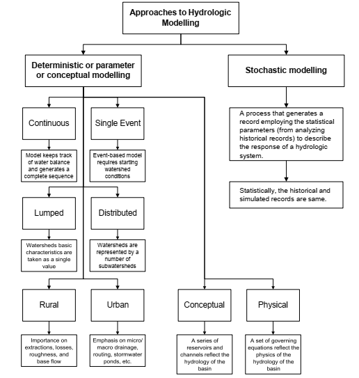
Figure 5.5 - Hydrologic modelling approaches.
Text version
Flow chart showing approaches to hydrologic modelling.
Deterministic hydrologic modelling allows for the construction of a system of physics-based relationships that are used to simulate the water budget within a basin and estimate flows. These models are typically used to generate a certain output (e.g., flow) for a defined set of initial conditions and specified meteorological forcing. As indicated in Figure 5.5, the selection of a model is dependent on the processes being simulated, data availability, design criteria, basin characteristics, and type of basin configuration. Once the modelling platform and model are selected, the next steps follow Figure 5.6 and are elaborated further in Section 5.5.4.
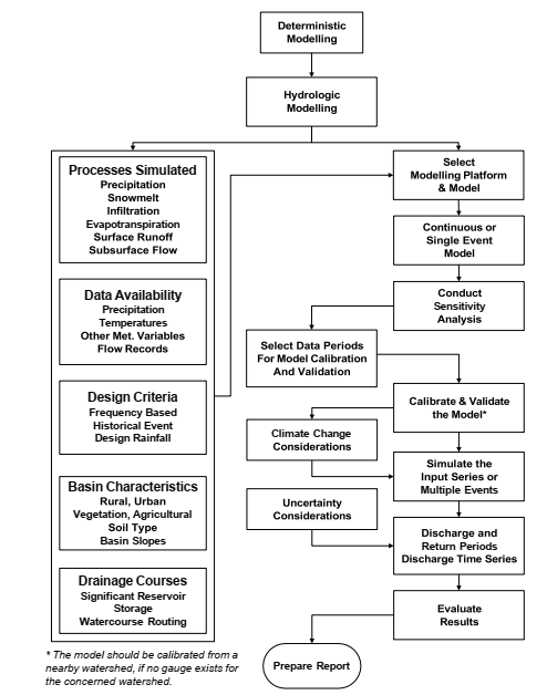
* The model should be calibrated from a nearby watershed, if no gauge exists for the concerned watershed.
Figure 5.6 - Deterministic hydrologic models.
Text version - Figure 5.6
Flow chart showing the next steps to follow once the modelling platform and model are selected.
Design flows resulting from a design storm input can be determined from single event models or continuous simulation models. Some available deterministic models can also be used in either single-event or continuous-simulation mode. Most hydrologic models used for the estimation of design flows require calibration and validation steps using observed sets of flow and model parameters of the basin. This process helps provide the best possible simulation results and is detailed in Section 5.5.4.
Continuous simulation hydrologic models generate long duration “synthesized or modelled” streamflow data for a watershed using various types of long-term meteorological records as inputs. The output is subsequently subjected to a single-station flood frequency analysis.
Probabilistic or stochastic models or techniques can be used to generate a set of outputs with associated probabilities for a range of possible input conditions. This type of model is often run as a Monte Carlo simulation, in which output probabilities are calculated based on a high number of model runs (e.g., over 1,000). Probabilistic models can quantify uncertainty in input conditions and are powerful tools for situations where input variables are uncertain; however, these models are not currently as widely used in hydrologic assessments as deterministic models. Vogel (2017) illustrates how deterministic hydrologic models can make use of stochastic meteorological series to generate ensembles of potential future streamflow that can also provide estimates of its variability. Such ensembles could be generated to reflect anticipated changes in climate and can inform flood hazard assessments.
5.5.1 Choice of Model to Use
Hydrologic models should be chosen based upon an assessment of appropriateness, including considerations of available input data, computational methods, and desired outputs. It may be necessary to use a combination of models for a specific task. Hydrologic models should also be of appropriate complexity to capture the dominant and sensitive processes in the modelled system. Scale is also an important consideration in hydrologic model applications. Other considerations include distributed versus lumped modelling approaches, and the methods of watershed routing (hydrologic versus hydraulic) within the modelling framework. Models that are inappropriate for the regime or scale being considered may introduce high levels of uncertainty. Reasons for model selection should be documented.
5.5.2 Continuous Simulation Modelling Using Long-Duration Meteorological Records
Continuous simulation hydrologic models are used to generate long-duration synthetic streamflow estimates for a watershed using long-term meteorological records as inputs. These may vary in complexity, but all track the state of a water budget within a basin over time. When a rainfall or snowmelt event occurs, these models use state variables, such as antecedent moisture conditions, and calculate the amount of discharge resulting from the event. Some models use a simple, continuously updated antecedent precipitation index to track watershed state between events. Others use a complex model of interception storage, soil moisture storage, groundwater storage, etc. Similarly, some models require only limited input data, such as precipitation and temperature, whereas others require many types of input meteorological data (e.g., precipitation, temperature, evaporation, transpiration, wind speed, dew point, cloud cover, solar radiation, etc.).
Assuming the model provides a good representation of the modelled watershed’s characteristics and has been satisfactorily verified (i.e., calibrated and validated), the synthesized flows can be used as though they were observed flows for further analysis. For example, they can be used in a single-station FFA to obtain design flows for various AEPs or used within a regional flood frequency analysis. However, there is a portion of uncertainty in these synthetic design flows that is difficult to quantify as the model will never be a perfect representation of the watershed’s characteristics, or of nature’s processes.
A more limited use of a simple continuous simulation model is to generate antecedent moisture estimates for a detailed single-event model. This can also be referred to as a “quasi-continuous simulation” approach.
5.5.3 Single Event Modelling Using Historical Storms and Design Storms
Single-event models generally use a time-distributed precipitation input, referred to as a hyetograph, to generate a time-distributed discharge output, or hydrograph. The input hyetograph will generally be either an observed historical storm or a synthetic storm using a typical rainfall distribution with a volume corresponding to a specific probability (e.g., 1% AEP) and duration (e.g., 6 hours).
Historical storms are recorded extreme storms that are used as inputs to hydrologic models. Such storms are dynamic events that move across watersheds. The areal extent of historical storms and their movement are important considerations in modelling.
Historical storms often exceed the minimum design criteria (e.g., 1% AEP flood) in a particular jurisdiction and for which precipitation data is available. In some Canadian jurisdictions, historical storms are used for regulatory purposes instead of design floods; examples are Hurricane Hazel in the Toronto area and the Timmins Storm in parts of northern Ontario.
Design storms have precipitation hyetographs generated by analysis of historical climate data. They are generally applied uniformly across an entire study area without allowing for spatial variation of the geographical features of the basin. Given the nature of this approach, its application is usually limited to small basins (NRC, 1989).
Design storms can be synthesized for specific watersheds and areas using local intensity- duration-frequency (IDF) curves. The most common example would be the “Chicago Storm”, which combines intensities at all durations for a common frequency. Other synthetic storm distributions are available for different regions of Canada. Common examples include the Soil Conservation Service (SCS) storm series and the Canadian Atmospheric Environment Service (AES) storm series. These storms are based on historical observations indexed to a particular duration (e.g., 24-hour rainfall for the SCS storms) and may not match the IDF curve at all durations. Caution is required to ensure that precipitation intensity at critical durations is represented appropriately.
A design storm with a particular AEP will not necessarily produce a flood hydrograph with the same AEP because different initial or antecedent conditions (e.g., soil moisture and water levels) will produce different flood responses. Modifying the initial hydrologic conditions can result in dramatically different design flows (Adams & Howard, 1986). An assumption regarding initial condition is needed to derive the design flows from the design storm, and these are sometimes set by the jurisdiction. It can be difficult to confirm and replicate those initial or antecedent conditions when conducting modelling.
5.5.4 Modelling Considerations
Figure 5.7 indicates that, irrespective of the time frame of the model, the hydrologic modelling procedures are the same, from these options:
- The simulation is a single event where the assumption that the AEP of the resultant peak flow is the same as the AEP of the event.
- The simulation is over a continuous length of time, such that an FFA uses the resulting annual peaks or peaks above a threshold.
- The simulation is of a series of storms, also requiring an FFA of the resulting peaks. The procedural steps for all options should be those in the bottom box of Figure 5.7.
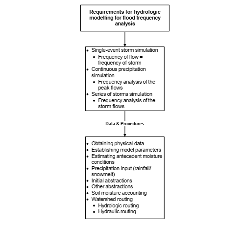
Figure 5.7 - Requirements for hydrologic modelling for flood frequency analyses.
Text version - Figure 5.7
Flow chart showing the requirements for hydrologic modelling for flood frequency analysis.
Considerations in model selection should follow elements of the flow chart in Figure 5.7 and include:
- Land use, including impervious areas and effects of deforestation, wetland drainage, and urbanization. Land cover significantly impacts infiltration rates and hydrologic response time. If planned or future land use differs significantly from current land use, this will produce a different design flow result.
- Appropriate discretization of the watershed into subwatersheds to capture the variations of land use, soil types, slopes, etc. and the number of flow computation points desired.
- The role that snowmelt plays in the hydrology and the degree to which the model can simulate snow-related runoff.
- Losses and gains from the modelled system, including groundwater inflows and outflows or inter-basin transfers. These should be modelled to the level of complexity necessary to adequately reflect hydrologic processes influencing the estimate of the required design flow.
- Routing of flows from the upstream subwatersheds downstream through the subwatersheds of the model.
- Inputs from upstream routing (e.g., channels and sewers carrying flows from upstream watersheds).
- Storage areas, such as behind culverts, dams, or in tailings and stormwater management ponds requiring volumes, inflow, and outflow rating curves.
- Model time-steps, which are chosen to allow for reasonably smooth progression of streamflows and should be short enough to capture peaks. For channel routing and reservoir routing, time-steps must be short enough to meet criteria for numerical stability for the given model. However, time-steps that are too short will increase computational time without appreciably increasing accuracy or precision.
When selecting the appropriate hydrologic model, data availability is an important overriding consideration.
5.5.5 Model Evaluation
A hydrologic model is a simplified mathematical representation of physical processes that can be used to predict the magnitude and rate of flow of water for a basin. To be useful, a hydrologic model should produce results that are acceptable based on model calibration (see Section 5.5.4), the model evaluation procedure, and the intended use of model outputs.
A numerical model is deemed verified for its intended purpose if it accurately represents the intended concepts and if it can produce reasonable and reproducible results. Models that are verified are not necessarily the best or most useful models; rather, they are judged to be applicable for their intended modelling purpose. Models are usually verified with existing observations; however, in some cases, no recorded matching streamflow and meteorological observations are available. In those cases, the model may be verified with a proxy watershed of similar hydrologic characteristics to determine the model parameters to use for the study site.
Figure 5.8 summarizes the steps used to assure the acceptability of the results of a hydrologic model. The first step is to examine the data used to characterize the watershed through a sensitivity analysis, to determine which parameters will most affect the flow from the model. The second step is to separate the streamflow data into calibration and validation sets. The calibration set of streamflow data will be compared to the model flows as the parameters are adjusted, while the validation set will verify that the adjusted parameters still produce a reasonable facsimile of the recorded streamflows. The third step is to determine how sensitive the model is to variation of the model parameters around the assumed mean values. Knowing which parameters are the most sensitive, adjust those parameters to calibrate the model. Verify the model fully with the validation set of streamflow data using the parameter values from calibration. The results from this simulation should meet the evaluation criteria set out at the beginning of the modelling effort. There are several evaluation criteria for hydrologic models, like:
- How well the mass balance is preserved over an event (i.e., precipitation volume less losses should equal volume of runoff, converted to the same units).
- How well the observed peak flow and computed peak rates compare.
- How well the time of peak flow rate of computed flow compares with observed timings, advanced or delayed.
Depending on the study objectives, two of the three noted criteria may suffice. If the objective is flood forecasting, the timing of the peak and a flooding threshold are the main focus; for the design of hydraulic structures and drainage pipes, peak flow rates and the volume of the design event are likely important parameters. While for delineating the flood hazard areas, the basic criteria are the peak flow rates to provide the maximum extent of flooding for regulation purposes.
The fully validated model is run with the design precipitation series and optimized watershed parameters to produce the design flows or using the projected future climate meteorological parameters, described in Section 4.0, and known future land cover conditions to allow for the incorporation of these non-stationarities. At this point, practitioners should analyze and interpret the resulting streamflows for the design frequencies to include in the hydrology report as described in Section 10.0. The hydraulic analyses may simulate the resulting design flood flows in a hydraulic model to determine the extent of the flood hazards.
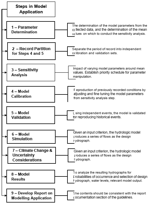
Figure 5.8 - Steps in model application.
Text version - figure 5.8
Flow chart showing the steps in model application.
- 1 – Parameter Determination
- The determination of the model parameters from the collected data, and the determination of the mean values on which to conduct the sensitivity analysis.
- 2 – Record Partition for Steps 4 and 5
- Seeparate the period of record into independent colibration and validation sets.
- 3 – Sensitivity Analysis
- Impact of varying model parameters around mean values. Establish priority schedule for parameter manipulation.
- 4 – Model Calibration
- Feproduction of previously recorded conditions by adjusting and fine tuning the model parameters from sensitivity analysis step.
- 5 – Model Validation
- Using independent events, the model is validated for reproducing historical events.
- 6 – Model Simulation
- Given an input criterion, the hydrologic model produces a series of flows as the design hydrograph.
- 7 – Climate Change & Uncertainty Considerations
- Given an input criterion, the hydrologic model produces a series of flows as the design hydrograph.
- 8 – Model Results
- To analyze the resulting hydrographs for robabilities of coccurrence and selection of design ydrograph, water levels, relevant model output.
- 9 – Develop Report on Modelling Application
- The contents should be consistent with the report cocumentation section of the guidelines.
Additional details on the steps described in Figure 5.8 are provided below:
- Parameter Determination: Based on the model proposed for generating design flows, decide which parameters in the models are fixed and which are variable to set the framework for the verification process, starting with the separation of the period of record and sensitivity analysis (see Step 2 below). Any assumptions made at this step will need justification in the report.
- Record Partition: Calibration and validation sets should each contain different hydrographs of high flows to compare the observed hydrographs with those simulated by the hydrologic model. Not all input and output data should be used for calibration; a subset of data should be set aside for validation. The World Meteorological Organization (WMO) has provided guidance on the amount of data that should be used for calibration of continuous simulation models versus that which should be reserved for validation (WMO, 2011). Other organizations have also refined those guidelines to define the number of events to be used for calibration and validation for event-based models.
- Sensitivity Analysis: Internal model parameters including runoff coefficients, snowmelt factors, and other variables are modified through an input range of reasonable values to determine the sensitivity of the model to these parameters. Parameters that show a high level of sensitivity are chosen using robust and documented methods or, in the absence of such methods, assigned values suggested in model documentation.
- Model Calibration: Models are calibrated using known input and output data. For example, if precipitation inputs and downstream streamflows are known, internal model parameters, such as runoff coefficients and snowmelt factors, can be adjusted to achieve model calibration. Individual model calibration efforts may not match both peaks and volumes exactly for every event, and it is unlikely that single calibration efforts will result in calibrated models that accurately capture floods derived from different flood mechanisms (e.g., spring freshet versus short-duration pluvial flooding). At the onset, practitioners must decide which aspect of the simulation is most important to get accurately.
- Model Validation: The calibrated model is validated for its intended purpose(s) by running the calibrated model using the set-aside validation input data to again compare modelled versus measured output data for the second set, for the simulation aspects that the model was calibrated to capture well.
- Model Simulation: Use the meteorological input of the design criterion (e.g., design storm for a prescribed AEP or a historical storm) or pass a long period of meteorological data through the model to obtain synthetic flow data as input for an FFA to obtain the design flow.
- Climate Change and Uncertainty Analysis: Apply the future meteorological parameters determined in Section 4.0 that consider climate change. As further explained in Section 9.0, the uncertainty analysis includes an assessment of potential sources of uncertainty including those associated with parameter values, hydrologic constants, input data, and methods. This analysis can be performed using numerical modelling or more qualitatively by considering the results of sensitivity analysis, input data representativeness, and goodness-of-fit for model calibration and validation.
- Model Results: Evaluate the results of the application of FFA to the series of simulations of a long meteorological record to determine the design frequency event, the simulation of climate change meteorology, or the simulation of a design storm to determine the design hydrograph(s) to use in the hydraulic analysis (Section 6.0).
- Report: Fully document the hydrologic modelling procedures used to assess the design flow as listed in Section 10.2.
Practitioners need to evaluate the performance of a hydrologic model simulation that uses these steps with comparisons to flows derived by other methods. This evaluation requires good professional judgment and a robust approach. Qualified reviewers not involved in the project may perform the evaluation.
5.6 Evaluation of Results
It is important to ensure that the recommended design flow for outlining the flood hazard area is grounded through supplemental and tertiary verifications through alternate methods. For example, if the design flow is computed through hydrologic modelling, then alternative estimates from regional methods should be obtained. Similarly, if FFA is the basic technique, then regional estimates from the index and multi-regression methods will provide alternative estimates.
Interpretation and rationalizing will be an important step at this stage. It is equivalent to the triangulation technique used in surveying to minimize the error on closure.
5.7 Reporting Requirements
Practitioners should fully document the design flow or water level assessment process, as detailed in Section 10.0. This document will explain the input data, why certain procedures were chosen over others, the software used, any difficulties encountered and how they were overcome, and the review process. The report will present the resulting design flow or water level assessment.
5.8 Summary of Hydrologic Procedures
The estimation of the design flows are inputs to the hydraulic analysis that will generate the extent, depth, and velocities of flooding. Therefore, the validity of the flood hazard delineation is only as good as the estimate of the design flows. The hydrologic procedures outlined in Section 5.0 should provide the best possible design flows, whether by an FFA or an RFFA of suitable historical recorded streamflows or water levels, or a calibrated and validated hydrologic model. A thorough review of the methods used by qualified reviewers not involved in the project should precede the hydrology report documenting the data used, the selection of the analytical approach, and the evaluation and uncertainties of the results.
6.0 Hydraulic Analysis
The purpose of hydraulic analyses is to simulate the effects of flows, winds, waves, ice conditions, and other hydrometeorological and physical factors on water levels of a waterbody, its surrounding flood hazard area, and at the water-land interface. As a result, hydraulic models produce the data necessary to develop inundation maps, to illustrate the depths, velocities, and extents of flooding.
This can be a more sophisticated process than was possible during flood hazard delineation programs conducted in the 1970s and 1980s, thanks to advancements in hydrodynamic research and numerical model development, and because computers have become more powerful and are better able to compute more complex aspects of flow dynamics. Also, significant advancements in the availability and reliability of topographic survey data can provide a much more detailed and accurate picture of the channel and flood hazard area surface. These include the collection of digital terrain models (DTM), bathymetry data by sonar-based technologies, and land surface elevation and land-use information using LiDAR and other forms of remote sensing.
The complexity of the hydraulic analysis should be commensurate with the data available and the project objectives. A more complex modelling platform will not necessarily increase the accuracy of results if there are limitations in the estimates of flows or other hydrometeorological variables, or in the topographic data used to construct the model; rather, more uncertainty will result. If the project covers densely developed areas, more complex modelling will be necessary than projects defining flood mapping for undeveloped areas.
Section 6.1 further explains modelling techniques in a fluvial context—both with a steady-state analysis, which simulates constant flows to determine the extent and velocities of inundation, and also with unsteady-state analysis, which can simulate temporally and spatially varying flow hydrographs and water levels, and which can additionally determine the duration of inundation. Section 6.2 discusses inputs to hydraulic models, while Section 6.3 discusses model calibration and validation.
A description of fluvial hydraulic practices is included in this section; individual tasks are described in Table 6.1 and cross-referenced to the procedure flow chart provided in Figure 6.1.
| Hydraulic Practices | |
|---|---|
| Step 1 | Determine modelling objectives, spatial extents, relevant hydrometeorological factors, and accuracy constraints based on the municipal, provincial, or territorial mandates and land-use planning and development policies. Define the floodway and flood fringe using the appropriate guidelines in each jurisdiction. |
| Step 2 | Assemble and review existing hydrometric and topographic data. Identify hydraulic data from all sources in the defined study area that meet data requirements. Document data sources. Conduct a QA/QC check on all hydraulic data used in the analysis. |
| Step 3 | Select platform for numerical modelling. The selection of analytical methods and models depend on the input data available, the analysis to be conducted, and the output data required, as well as on professional judgment, expertise, and model availability. |
| Step 3a | Use 1-D models when channel and overland flow are uniform and velocity can be reasonably assumed to be parallel to stream channels. |
| Step 3b | Alternatively, employ 1-D steady-flow modelling in uniform reaches combined with 2- D modelling, where restrictions and channel curves render flow more complex, with some velocities perpendicular to the stream channel. |
| Step 3c | Alternatively, use 2-D and quasi-2-D modelling when channel flow is relatively complex, when other hydrometeorological factors (e.g., winds) are relevant, where velocities are not assumed to be perpendicular to stream cross-sections, and to model complex overbank areas, including urban areas, areas with dikes and other flood-protection measures, and areas where different scenarios will be modelled (e.g., dike breach). |
| Step 4 | Identify data gaps and required data collection. Streamflow and water level data will verify the model; topographical data at culverts, bridges, dikes, and flood hazard areas will better define the hydraulics of the flows. |
| Step 5 | Select varied, but generally high streamflow and water level data periods for model calibration and validation. Use two distinct sets of corresponding streamflows and water levels, one for calibration, and the second for validation. Consider the reliability of the data, including its accuracy, the time period it was collected, and external factors that may impact its homogeneity and applicability to potential future events. |
| Step 6 | Conceptualize, conduct sensitivity analyses, calibrate, run, and validate the model.
|
| Step 7 | Compute flood depths, extents, and velocities from the hydraulic modelling of the design event(s) based on hydrologic analysis. Run the model with the various design AEP flows and future flows incorporating climate change. |
| Step 7a | Evaluate results by comparing, where possible, with recorded high-water marks, historical floods, and the streamflow record. Redo if unsatisfactory. Have qualified reviewers not involved in the project review the analysis. |
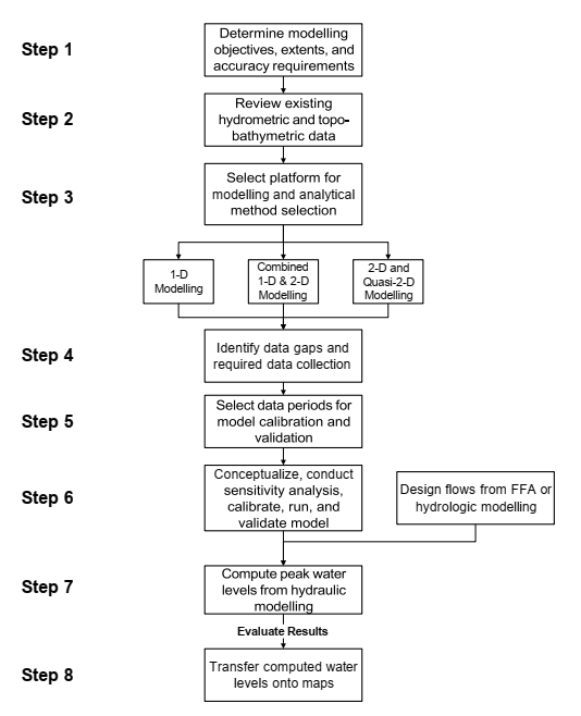
Figure 6.1 - Hydraulic modelling procedure.
Text version - Figure 6.1
Flow chart cross-referencing steps for hydraulic modelling procedures.
6.1 Model Selection
In general, fluvial hydraulic models for flood hazard delineation include modelling the main channel and the flood hazard area. This section details the various configurations of hydraulic models that practitioners could choose to meet the best option for the project’s objectives. For example, Table 6.2 provides a framework of the capability of the hydraulic models for various applications. Most hydraulic models are based on the finite difference solution of the Saint- Venant equations for one-dimensional (1-D) or the shallow water equations for the two- dimensional (2-D) flow. These equations define the principles of conservation of mass and momentum balance in a fluid. As noted, before, they are sometimes simplified in hydraulic models to exclude various terms in the equations. A comparison between 1-D and 2-D hydraulic models is provided in Table 6.2 (adapted from Pender, 2006).
| Method | Description | Application | Outputs |
|---|---|---|---|
| 1-D Steady State |
|
|
|
| 1-D Unsteady State |
|
|
|
| Quasi-2-D |
|
|
|
| 2-D |
|
|
|
| Combined 1-D & 2-D |
|
|
|
Commonly used hydraulic models in Canada include (in alphabetical order):
- 1-D riverine modelling: HEC-RAS, MIKE11
- 1-D riverine + urban modelling: Infoworks, MIKE+
- Combined 1-D & 2-D riverine modelling: HEC-RAS, MIKE Flood
- 2-D riverine modelling: HEC-RAS, Infoworks 2D, MIKE21, SOBEK, TELEMAC, TUFLOW, H2D2
- 2-D coastal/lake modelling: ADCIRC, Delft3D, MIKE21/3, TELEMAC
HEC-RAS is available from USACE (2021). MIKE11, MIKE+, MIKE Flood, MIKE21 and MIKE21/3 are available from DHI (2017). Infoworks in both versions is available from Autodesk (2020). SOBEK and Delft3D are available from Deltares (2020). TUFLOW is available from TUFLOW (2020) and TELEMAC is available from TELEMAC- MASCARET (2021). Luettich and Westerink (2016) maintain the ADCIRC model. H2D2 is available from INRS-ETE (Leclerc et al., 1998).
Modelling approaches include steady and unsteady 1-D, 2-D, quasi-2-D, combined 1-D and 2- D, and, in specialized cases, 3-D models. Hydrodynamic models used for lakeshore areas are described in Section 8.0.
6.1.1 1-D Steady-State Flow Modelling
Use of 1-D steady-state modelling is widespread and has been common practice in flood modelling/mapping activities for decades. It is intended for calculating water surface profiles for steady-state flow, that is, where it may be assumed that flow rates change gradually, and the hydraulic profile may be accurately computed using flows that change spatially, but not temporally.
The basic computational procedure for this type of model is based on the solution of the 1-D energy equation. Energy losses are evaluated as the sum of friction, contraction, and expansion losses. The momentum equation may also be used in situations where the water surface profile is rapidly varied, such as at bridge openings, and when evaluating profiles at stream confluences.
A 1-D numerical model is based on the following assumptions (Cunge et al., 1980):
- Flow is largely confined and one-dimensional in the direction of the main channel.
- Flow is perpendicular to the channel cross-sections.
- Water levels across the channel cross-sections are uniform and do not vary.
- Vertical accelerations are negligible.
- Effects of boundary friction and turbulence can be accounted for using resistance laws analogous to those for steady flow conditions.
- Average channel bed slope is mild.
This type of model is relatively simple to set up and run, does not require powerful computer processors, has lesser data requirements than more complex alternatives, and is capable of efficiently generating accurate results for streams that meet the listed criteria when applied by experienced practitioners. These models do not require full stream bathymetry and are particularly good at modelling in-stream features including culverts, bridges, weirs, dams, and other hydraulic structures.
The scale of the results is suitable for design over a channel reach in the order of tens to hundreds of kilometres.
In general, 1-D steady flow modelling requires the following inputs:
- Peak flow for the steady-state profile
- Input and lateral flow hydrographs
- Stream cross-section shape information (elevations)
- Bank stations
- Hydraulic structure information
- Hydraulic coefficients (e.g., expansion and contraction)
- Channel resistance coefficients (e.g., Manning’s roughness)
- Rating curves
- Boundary conditions
6.1.2 1-D Unsteady Flow Modelling
Applications for 1-D unsteady flow modelling, also known as 1-D hydrodynamic modelling, include model situations with changes in storage, flow reversals, variable boundary conditions, rapidly varying flow and waves (e.g., dam breaks, flash floods), and the need to understand the interaction with time-varied flows from tributaries. This type of modelling has been less common than steady-state 1-D modelling in the past but is used more frequently today thanks to faster computational speeds and the need to model more complex phenomenon, such as variable flow rates along a channel that result from channel storage and flood wave attenuation. The scale of the results is suitable for a channel reach in the order of tens to hundreds of kilometres. If only sparse cross-sectional data is available, the hydrodynamic model will only provide broad-scale results.
The data requirements for most 1-D hydrodynamic models are similar to 1-D steady-state models, with the exception of the need for appropriate time-varying boundary conditions and hydrographs, which give the variation of flow over time.
6.1.3 Quasi-2-D Modelling
Quasi-2-D modelling involves linking multiple 1-D models together to account for overland flow separately from the main flows. Although this method can involve setting up several distinct models, the individual models are generally simple and model outputs from upstream segments are used as inputs for downstream segments. This method has been shown to require less computing power and have similar accuracy to 2-D modelling, when properly configured. Its application is restricted to broad-scale modelling.
6.1.4 2-D Modelling
In some practical situations, the interaction of channel and flood hazard area flow fields is quite complex, including situations where the stream banks are poorly defined, flow attenuation and flood hazard area storage is important, and flow properties are complex (e.g., along streets and between developments). For these applications, 2-D hydraulic models are generally preferred (Horritt & Bates, 2002; Hunter et al., 2008).
The 2-D models employ depth-averaged Navier-Stokes equations, commonly called the shallow water equations, which allow for the simulation of horizontal components of the flow velocity in two directions and which can produce more realistic results for complex flood situations if properly configured with sufficient data. These models are particularly suitable when detailed information about flow velocities and depths is required, flow-depth and local velocity hazards to people and property are important, and for which lateral variation in water surface elevations are important. The criteria for using 2-D modelling are listed in Table 2.2 as well.
Most 2-D models are typically more complex and take more time and greater levels of experience to develop, calibrate, and validate than 1-D models. These models require longer simulation times than 1-D models, but thanks to continuous improvements in computing resources, the time and cost requirements of 2-D modelling are decreasing.
In terms of data requirements, detailed digital elevation models, such as LiDAR data, and full bathymetry (rather than stream cross-sections) for stream channels, are generally required to support 2-D modelling. The data requirements may limit the scale of the results to a reach in the order of tens of kilometres. Data and grid-resolution may also be a limiting factor. For example, if applying a coarse elevation spatial grid, a 2-D hydrodynamic model may only provide broad- scale results.
6.1.5 Combined 1-D and 2-D Modelling
A potential solution to the greater computational demands and data requirements of 2-D modelling involves the use of combined 1-D and 2-D modelling. This usually involves using 1-D models for the defined flow channel coupled with a 2-D model in the complex overbank areas. There are a number of hydraulic modelling software packages that allow the coupling of 1-D and 2-D models. The advantage of using a combined 1-D and 2-D model is that the model is simpler, faster to run, and allows the advantages of both 1-D and 2-D modelling to be applied where appropriate and as needed. However, this comes at the cost of increased data requirements, increased model complexity, greater resources to develop and calibrate, and longer simulation times compared to 1-D modelling.
6.1.6 3-D Modelling
In addition to the horizontal velocity component achieved using 2-D models, 3-D models include a vertical velocity component. These models are generally used for water-quality studies, such as water intakes and outfalls, where density stratification (e.g., due to salinity, temperature, or suspended sediment concentration gradients) affects the movement and mixing of water.
The use of 3-D models is uncommon in flood hazard studies. For some specialized cases, complex 3-D models known as computational fluid dynamic (CFD) models may model flow through or around an engineering structure (e.g., dam spillway, sluices, etc.).
6.1.7 Physical Models
Physical models were generally used by organizations with specific technical needs to evaluate conditions that may not be well represented by computer models, and to use simulations to obtain empirical data about real-world processes. A high level of expertise and resources are required to design experiments that properly account for scaling.
6.2 Data Requirements
6.2.1 Geospatial Data
The accuracy and precision of hydraulic analyses and flood hazard maps is highly dependent on the quality of geospatial input data used. The Federal Airborne LiDAR Data Acquisition Guideline (NRCan and PSC, 2018) and the Federal Geomatics Guidelines for Flood Mapping (NRCan and PSC, 2019) provide guidance on sourcing and using geospatial data for flood mapping.
Geospatial data may include stream cross-sections (generally to support 1-D modelling) or detailed continuous digital elevation models and bathymetry (generally to support 2-D modelling).
6.2.2 Stream Cross-Sections
Stream cross-sections are the basic input to 1-D models. They are usually gathered from ground-based surveys and/or extracted from a combination of continuous bathymetric and LiDAR surveys. The cross-sections should be representative of the typical topography and cross-sectional area available for a particular reach. Cross-sections should be taken perpendicular to the direction of flow and across the full width of potential inundation, without crossing each other. Some models suggest the cross-sections be bent in the overbank areas to maintain the cross-section perpendicular to the flow. This approach must be used appropriately to prevent an overestimate of the flow area and to maintain stream channel length.
Cross-sections should be located to capture significant changes in channel characteristics, such as channel width and bed slope, and to define abrupt changes that result from weirs, bridges, culverts, and other hydraulic structures. Take cross-sections above and below hydraulic structures and significant inputs (e.g., tributaries, storm sewer outflows, etc.).
6.2.3 Bathymetry and Digital Terrain Models
A continuous, more detailed characterization of the channel and overbank topography is required for 2-D models, and if available, can also be used to extract 1-D cross-sections from a channel. This typically includes a combination of bathymetric data in the main channel and LiDAR or ground-based survey information for the overbank areas, which are used to create a continuous model of the riverbed and land surface, that is, a digital terrain model (DTM).
This topography data is represented as either a regular or irregular grid in three-dimensions. The grid is described by nodes, the location of which are entered as horizontal map coordinates with corresponding elevations determined from the channel bathymetry or overbank topography for the entire extent of the modelled body of water. Information on previous flood extent may provide guidance on the spatial extent of the DTM required, but consideration should be given to potentially greater flood events in future events.
Grid resolution required depends on the application. The finer the grid, the greater the computational requirements; however, a coarser mesh may not be able to accurately represent the turbulence of flows at complex points in the topography. At those points, such as at a sharp turn, outflow, or bridge abutment, the grid resolution should be increased.
6.2.4 Resistance Coefficients
Most hydraulic models require the selection of coefficients that help describe the energy losses due to the channel resistance (i.e., roughness or friction). Various researchers have developed a number of these coefficients. For the purposes of these guidelines, discussions are limited to the use of Manning’s “n” in the open-channel flow modelling.
Manning’s roughness, “n”, is one of the most common coefficients, which derives from Manning’s well-known open-channel empirical flow equation. Manning’s roughness allows for modelled stream conveyance to be altered based on the physical characteristics of the stream channel and overland flow area, such as bed material, vegetation, seasonality, and other features that are in contact with flow. In modelling applications, roughness coefficients can also surrogate for limitations and uncertainty in the representation of other channel characteristics.
Manning’s roughness is an empirical value that not only varies with the physical stream roughness, but also with its relationship to stage and flow. There can also be seasonal changes in roughness, particularly in overbank flow areas. In practice, several different Manning’s roughness coefficients may be used in a single hydraulic model, with potential variations occurring across individual single-stream cross-sections and at different cross-sections.
Selecting the appropriate resistance values requires an understanding of stream hydraulics, and care should be taken to select reasonable values that consider both physical characteristics of the system and requirements for a hydraulic model.
It is likely that initial resistance coefficient values will be altered during the calibration process, but calibration should not be forced by choosing values outside a reasonable range of values. Increasing channel resistance for a stream reach will decrease the flow velocity and therefore locally increase the stage while increasing flood wave travel time. The relationship between flow rate and flow stages is somewhat sensitive to changes in channel resistance and the appropriate values should be selected based on a thorough understanding of the model and how the coefficient is used, a review of the pertinent literature, and hydraulic expertise.
Initial resistance coefficients may be selected using one of the following references:
- Consultation with published Manning’s roughness values (e.g., Chow, 1959).
- Comparison to similar streams with calculated Manning’s roughness values (e.g., USGS, 2017).
- Equations specifically intended to relate Manning’s roughness to physical stream properties (e.g., Limerinos, 1970).
- Using technical expertise from hydraulic experts familiar with the studied stream.
In all cases, the calibration and validation procedures may adjust the selected Manning’s roughness values, but they should remain within the limits set forth in the preceding references.
6.2.5 Hydraulic Structures
Hydraulic structures include weirs, dams, bridges, culverts, and other in-stream features. These structures can significantly alter streamflow characteristics, including velocities and water levels, and every effort should be made to model them accurately. If there are any policy implications on the presence of the hydraulic structures, these should be evaluated and their impacts on resulting flood line assessed.
Generally, design information on hydraulic structures is entered into a hydraulic modelling software program, and loss coefficients are chosen based on published values and professional judgment. If possible, losses at hydraulic structures should be checked using a second computation method. Calibration and validation should be completed over a wide range of flows. Generally, 1-D models are better for modelling hydraulic structures and losses than higher dimensional models, they also require less data and computational resources.
6.2.6 Dikes and Other Flood Mitigation Measures
Hydraulic analysis should include an assessment of the impact of dikes and other flood mitigation measures on flood stages. A river or stream that contains significant overland flow paths where large flow quantities leave the river at one point and re-enter downstream is another example requiring careful analysis. Due to the local impact on water levels, these features should be accounted for in the model conceptualization (e.g., urban flooding on a river that meanders through a city). Similar to the policy implications noted in Section 6.2.5, these should be evaluated for potential breach or flow around the dikes or other measures.
6.2.7 Boundary Conditions
The boundary conditions for the model depends on the nature of modelling, steady or unsteady. These specified boundary conditions should not adversely affect the simulation process. For example, for a steady-state, subcritical flow simulation, the downstream boundary of the model should be chosen so that the simulated water levels within the study area of interest are not sensitive to the downstream water level, where possible. This can be achieved by selecting a location sufficiently far downstream to have low sensitivity to upstream flows (evaluated by conducting a sensitivity analysis) or by selecting a control point at which the upstream reach is hydraulically independent.
Alternatively, an unsteady-state model should be selected that allows the boundary conditions to be altered during the simulation to produce a representative hydraulic profile. An example of this is simulating the influence of tides on water levels using a hydrodynamic model where the downstream water level boundary can change to represent ocean levels. In this type of simulation, initial boundary conditions should be chosen to be both physically realistic and to allow the flow rates to be gradually varied to prevent model instabilities. The model can also be allowed to “warm up” through steady-state modelling prior to the starting point of simulation.
In the case where the downstream boundary condition is variable, for example, it is controlled by the ocean, a large lake or by a much larger river (i.e., where flooding is governed by independent processes), the boundary conditions should reflect conditions that are reasonably likely to occur concurrently with the design flood on the study stream (e.g., high tides or seasonal peak water levels on lakes and rivers). There may be a transitory reach near the confluence of two water bodies (e.g., coastal estuaries) where the influence of boundary conditions on flood levels becomes significant. Joint probability analysis or long-term simulation using continuous data records may be necessary to establish flood levels in such transitional reaches.
6.2.8 Stage-Discharge Relationships
Stage-discharge relationships, or rating curves, describe the relationship between water level and discharge at a specific stream location (e.g., hydrometric station) and are often used as boundary conditions in hydraulic model applications. They are generally used to estimate discharge from a measured water level.
These relationships are usually derived by one of these methods:
- Conducting field discharge measurements at a range of water levels, plotting, or fitting the relationship curve to the measured data, and deriving the associated equation.
- Conducting stream cross-section measurements to determine stream profiles at specific locations.
- Conducting hydraulic modelling using a software program.
Estimating stream discharge at a hydrometric station based on measured stage allows a flow hydrograph to be developed that can be used as an input to a hydraulic model or to estimate historic high flows outside the period of record where only high-water marks are known for the calibration and validation steps. Crowd-sourced, academic science-derived measured flows, and/or water levels may also be related using applicable stage-discharge relationships.
Ice or vegetation in the channel, downstream blockages, and bed cross-sectional changes will alter the stage-discharge relationship. Flooding events can also alter the stage-discharge relationship and are an additional consideration in flood mapping and modelling activities.
6.3 Sensitivity Analysis, Model Calibration, and Model Validation
A hydraulic model, no matter how simple or complicated, needs to be calibrated and validated before it can be used reliably. Calibration is done by adjusting certain model parameters, such as Manning’s roughness, so that modelled water surface elevations match observed levels as closely as possible over a period of time or a series of events.
After the model is calibrated, a separate series of flow events not used for the calibration process are used to verify the predictive accuracy of the model (refer to Figure 6.2).
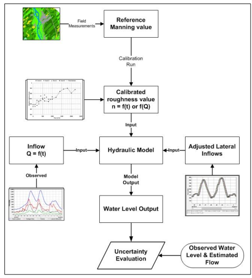
Figure 6.2 - Calibration and validation of a hydraulic model.
Text version - Figure 6.2
Flow chart showing the steps to calibrate and validate a hydraulic model
6.3.1 Sensitivity Analysis
The first step in calibrating and fully validating a fluvial hydraulic model is to determine where the results are the most sensitive from initial values assessed by field observations, user manuals of the models, and textbook examples. A list of potential model parameters should be prepared. The mean initial values are run by increasing or decreasing a model parameter and the changes are listed holding all other parameters constant. Once all model parameters are run, the list is prepared with the parameter of maximum changes to the water levels/flows first, ready for the calibration stage discussed below. These highly sensitive parameters will be modified first when calibrating the model. The sensitivity analysis may also determine the best location for the boundary conditions.
6.3.2 Model Calibration
Practitioners should run the model using observed water levels for calibrating the model. Selecting the study reaches where the model results are most sensitive to the roughness and hydraulic loss coefficients, practitioners should then adjust those parameters within published ranges from other similar projects to arrive at simulated water levels that are reasonably close to the observed ones for the similar flow conditions. Reasonably close, for example, is within 5 cm of the observed water levels or 10% of the computed flow.
If it is not possible to obtain water levels that match observations with parameters that are within reasonable limits, this may indicate there are problems with the topographic or boundary condition data. The tolerance for the difference between model results and observed values should be stated in the initial objective phase of the study.
For calibrating hydraulic models, consideration should be given to the following list and procedures developed by USACE HEC (Brunner et.al., 2020):
- Hydraulic roughness parameters
- Contraction and expansion coefficients
- Ineffective flow area extents and height trigger elevations
- Hydraulic structure coefficients
- Bend loss coefficients (sometimes called minor losses)
- Boundary condition information, such as energy slopes, or even potentially rating curve values
- Debris blockage information at structures
- Levee breach dimensions and timing values
A list similar to the one above results from a sensitivity analysis that prioritizes the importance of a model parameter on the output.
The modelling parameters that are most sensitive in previous steps (usually Manning’s roughness and the loss coefficients at hydraulic structures) are adjusted during the calibration of the model stage. Manning’s roughness is often lower with the higher depths associated with higher flows. Preferably, as a first step, practitioners should use higher observed flows to find the Manning’s roughness that yields model results closest to the corresponding observed depths and extents of flooding.
6.3.3 Model Validation
Once the simulated results fall within the defined tolerance limits, the next step, where data are available, is to validate the model with a second independent set of data to ensure the calibrated values produce acceptable results universally. The initial criteria for the procedure should set out how to evaluate the acceptability of the model results: whether within a tolerance or a percentage of depth and over which duration, whether the peak or the entire hydrograph. A statistical analysis may define the fit required to fully validate the hydraulic model. Furthermore, comparing the observed water levels with the simulated allows for an evaluation of the accuracy of the model. Procedures outlined in the HEC-RAS user’s manual (USACE, 2022) are good resources to review during model calibration and validation stages.
6.3.4 Fully Validated Model
Once calibrated and validated for the values of the roughness and loss coefficients with the two sets of observed levels and flows, the fully validated fluvial hydraulic model may simulate the design floods to determine the flood hazard extents, depths, and velocities.
6.4 Reporting Requirements
The documentation for the analysis covers the choice of model(s) and data used in the procedures for the fluvial hydraulic analysis. It should include tables of the parameter values after the sensitivity analysis, calibration and validation steps, and corresponding results comparing observed and simulated flows, water levels, and velocities, and that describe the accuracy of the model. Section 10.0 covers the detailed requirements of the report.
6.5 Summary of Hydraulic Procedures
The definition of the purpose of the hydraulic model for a flood hazard delineation, and to some extent, the available data, will guide the analytical method to use. The simplest possible hydraulic model may result in explaining a large percentage of the variance of the results. More complex models need increased data and parameter requirements. The hydraulic models will require the design flow(s), either as a constant peak (steady-state) or as a hydrograph (unsteady-state), and data on the channel bathymetry and overbank topography, either as two- dimensional cross-sections normal to the streamlines (for 1-D models) or as a three- dimensional grid or mesh points (for 2-D models). The resistance coefficients are empirically derived values used to describe roughness characteristics of the channel and overbank materials and the hydraulic loss coefficients of the infrastructure, though in practice they may also account for other sources of model uncertainty. These coefficients may be refined during model development and calibration. Full validation of the model incorporating those coefficients, comprised of sensitivity analyses, calibration, and validation, with observed values of depth and extent of inundation for recorded high flows, is necessary to ensure reliability of simulated model results. After that, the model may be used to simulate the effects of the design flow on water levels and velocities, and to delineate the flood extent and related hazards. Qualified reviewers not involved in the project should examine the analysis and results. The final model results are ready for presentation on flood maps for public information and a report as outlined in Section 10.0.
7.0 Ice Effects
Ice-related floods are complex physical processes that occur in many parts of Canada. As such, ice effects should be considered when conducting hydrologic and hydraulic assessments to support flood hazard delineation in riverine and lakeshore study sites. The primary cause of ice- related river flooding in Canada is ice jams, which can occur at freeze-up, at spring breakup, or during a breakup event triggered by a mid-winter thaw. Modelling ice-related flooding is a specific technical discipline and requires the involvement of experts (Kovachis et al., 2017; Lindenschmidt et al., 2018).
A description of procedures for considering ice effects in hydraulic analysis is included in this section. However, note that there is more than one potential method for assessing the probabilities and physical processes for ice-jam flooding. As such, reliance on a qualified professional for carrying out the ice analysis is necessary. A summary of processes leading to ice jams is provided in Figure 2.8. Potential individual tasks for ice impact analysis are included in Table 7.1 and cross-referenced in Figure 7.1.
| Ice-Jam Flood Assessment Practices | |
|---|---|
| Step 1 | Evaluate the study site to see whether it has experienced ice jamming or if it exhibits characteristics typical of ice jamming to determine if an ice-jam flood assessment procedure is necessary (Section 7.3). |
| Step 2a | If water level data for a period of 25 years or more is available, conduct an FFA of the known ice-influenced high-water levels to help determine the design high-water level (Section 7.4.2). |
| Step 2b | If insufficient data is available for direct determination, conduct a synthetic ice-stage frequency analysis using synthetic data generated by ice-jam mechanics (Section 7.4.3). |
| Step 3 | Check for stationarity. |
| Step 4 | Determine the probabilities of flood stages occurring from ice jams for the recorded or synthetic data (or combined data) to select the stages (water elevations) associated with the design AEPs (Section 7.4). Assess the impacts of climate change for the study site (Section 7.3.3). |
| Step 5 | Where a hydraulic model will be used to determine two-dimensional flows and velocities from design AEP ice-jam events, estimate the likely discharges that correspond to the selected stages of the design AEPs, using specific ice-affected stage-discharge relationships based on recorded relevant ice-jam conditions at the study site. Develop a site-specific hydraulic model under ice, from the many available, calibrating and validating with separate sets of recorded flood events under ice-jam conditions, after a sensitivity analysis. Conduct any uncertainty evaluation (Section 7.6). |
| Step 6 | Conduct a two-dimensional hydraulic analysis of the design AEP discharges to determine the ice-related AEP backwater effects using this ice-affected hydraulic model (Section 7.6). This analysis is complex and should involve experienced practitioners with relevant expertise. An independent review of the data, procedures, and outcomes should occur. |
| Step 7 | Map inundation extents under open water and ice conditions for selected AEPs. Document the procedure in a full report. |
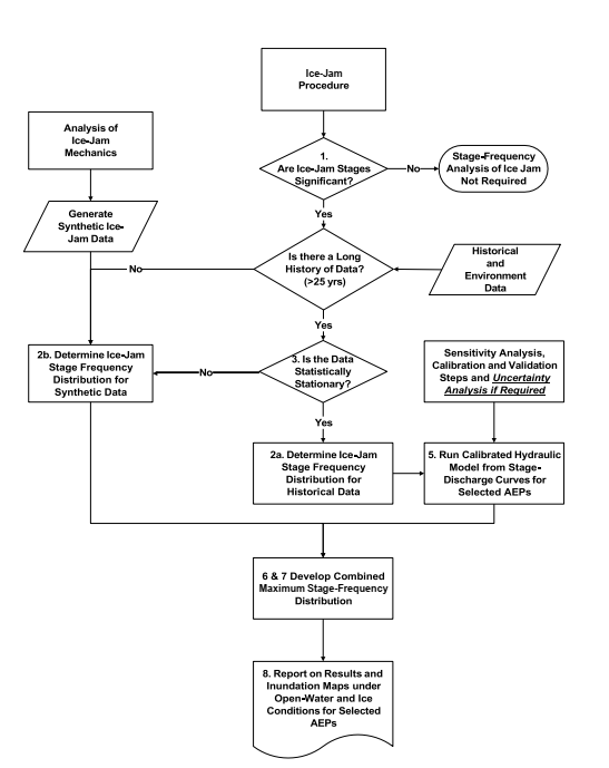
Figure 7.1 - Ice-jam procedure.
Text version - Figure 7.1
Flow chart showing the steps for a ice-jam analysis procedure
7.1 Ice-Related Flooding
There are currently two standard methods for incorporating ice-related impacts into flood frequency analysis (FFA):
- Conventional analysis, using direct incorporation of ice-affected flooding using stage- frequency analysis with long-term datasets that include several well-documented ice- affected flooding events.
- Synthetic frequency curve generation, based on an understanding of river ice mechanics and applications of simple probabilistic concepts (Beltaos, 2012) or Monte Carlo simulations for different defined ice-related events.
The annual ice-related peak water level may result from thick ice-cover roughness, a sudden release of water upstream (a “jave”), or most likely from an ice jam, which dominate in most years when ice-related high water occurs. Although ice jams tend to recur on specific reaches or known lodging points of certain rivers, the probability of an ice jam occurring, the timing of the ice jam, and the effect of the ice jam are difficult to determine. If possible, hydrometric data for ice-related events should be used directly to create an ice-affected flood frequency curve. When there is not sufficient ice-related data to directly calculate AEPs and extrapolate to rare events, synthetic frequency curve generation methods are possible, albeit entailing greater uncertainty than does the conventional analysis. In the cases where a less-detailed analysis is appropriate, a high-level preliminary assessment can provide a coarse estimate of the maximum expected ice-related levels.
7.2 High-Level Preliminary Assessment
In many cases, a simplified analysis of ice-related water levels is undertaken to provide a reasonable estimate of the maximum expected ice-related levels because it is not deemed to be important, open-water conditions are believed to govern, or there is insufficient data available to warrant an extensive analysis. In these situations, a suitable procedure would be as follows (Associate Committee on Hydrology, 1989):
- Assess the potential for the development of ice jams or severe ice accumulations based on geomorphic features (e.g., slope changes, channel constrictions, sharp bends, etc.) evident on maps and aerial and satellite photographs.
- Consult satellite imagery and other remotely sensed data to track ice conditions on a seasonal basis to characterize dominant processes locally and on a reach-scale.
- From site inspections, identify vegetal and morphological features that would indicate the height of ice action (but be cognizant of caveats pertaining to such evidence, per Associate Committee on Hydrology (1989).
- Collect relevant news articles, anecdotal evidence, and oral history about ice conditions from Indigenous knowledge, residents, and authorities and correlate it with the vegetal and morphological indicators.
- Assess the mitigation potential of flood hazard areas and relief channels to limit the height of ice action.
- Estimate the severity of ice-related flows from a regional perspective, if necessary.
- Estimate the channel slope and channel dimensions at bankfull (map slope and a rectangular representation of the channel would be appropriate) and calculate the expected height of an ice accumulation using appropriate hydromechanical relationships or their graphical approximation (Beltaos, 1983).
7.3 Ice-Jam Flooding
Certain river reaches in Canada are more susceptible to ice-related flooding than others. Analyses of study sites that have a documented history of ice-related flooding should include an assessment of the impacts of ice jams on water levels and AEPs. Sites that may not have a documented history of ice-related flooding, but have characteristics that may lead to ice jams, should be evaluated for ice-jam risk.
There are three main stages in the life cycle of river ice: ice formation, ice thickening, and ice breakup. Figure 2.8 in Section 2.0 identifies the ice-jam potential during each of the three different stages and the following subsections describe the stages further.
7.3.1 Ice Formation and Thickening
Ice cover that forms at freeze-up can typically be treated as ice jams or ice accumulations, of which there are two types: juxtaposed and consolidated. A juxtaposed accumulation forms by the juxtaposition of ice floes, one layer thick, when the approach velocity is low enough to prevent the floes from being drawn under the leading edge of a previously formed ice cover. A juxtaposed cover can also form between strips of shore (or border) ice. In these cases, internal stability is developed by the freezing between the floes of ice covers, known as interstitial freezing (Andres, 1999). The internal strength of the relatively thin accumulation formed by the interstitial freezing is sufficient to withstand the increasing shear and gravity forces on the lengthening accumulation.
A consolidated ice cover forms if a juxtaposed ice cover cannot form, either because ice floes are drawn under the leading edge, or there is insufficient interstitial freezing to maintain stability (Beltaos, 2013b). Consolidated ice covers can be viewed as granular structures (Beltaos, 1995), which form by different mechanisms:
- Hydraulically, by the “narrow-channel” jam stability criterion (Pariset et al., 1966) wherein the accumulation is thick enough that its leading edge is not submerged. Unless fortified by freezing effects or the channel width is very small, this type of jam is unstable and collapses to form a thicker jam, as described next.
- Hydromechanically, by the “wide-channel” jam stability criterion where accumulation thickness is controlled by the balance between the applied external forces and its internal strength derived from intergranular friction. This type of jam occurs much more frequently than the narrow kind, especially during breakup in unregulated rivers.
Generally, the wide-channel stability criterion will produce the highest water levels, followed by the narrow-channel criterion, and the juxtaposing ice cover will produce the lowest water levels. Should either a juxtaposed or consolidated ice cover become destabilized and collapse, the ice cover can further thicken. These freeze-up ice jams can cause a dramatic rise in water levels, particularly on regulated rivers that have increased winter discharges.
Additionally, “hanging dams” can form by transport and accumulation of frazil ice and occasional ice floes under an already formed sheet ice cover. This type of ice jam is not encountered frequently but can lead to flooding because the deposited ice can attain extreme dimensions under certain circumstances. Details can be found in Beltaos (2013b).
7.3.2 Ice Breakup
Increases in temperature, either during warmer winter periods or during springtime, affect the breakup of ice cover in two ways:
- Thermal degradation of the ice cover.
- Mechanical fracturing, mobilization, and breakdown into ice slabs and blocks via increased flows associated with higher runoff (rainfall and snowmelt) and groundwater inputs.
Generally, when thermal degradation dominates breakup, the risk of ice jams is low. This is common for cases when flows do not substantially increase during breakup. However, in cases where flows substantially increase and mechanical breakup processes dominate, the risk of ice jams and associated high water levels is higher. When ice jams release, they generate ice runs and sharp water waves, referred to as “javes”. If the downstream advance of the ice run is arrested by still-intact ice cover and/or other obstacle, new ice jams may form.
Javes are complicated hydrologic phenomena that are created by the formation and release of ice jams and are an important feature of the breakup process. Larger ice jams lead to larger javes travelling downstream. Unsteady flow, including javes, may produce higher water levels and thicker ice-jam accumulations than may be modelled using steady-state jam theory. Considerable research has been carried out to understand the characteristics of javes (Jasek, 2003; She & Hicks, 2005; Beltaos, 2013a).
7.3.3 Climate Change Impacts of Ice-Jam Flooding
Under the warmer temperatures seen now and expected in the future, most areas of Canada are anticipated to see later freeze-up and earlier spring breakup of ice-covered streams. A relatively thinner, weaker ice cover and increased winter flows under the predicted warmer climate would enhance freeze-up consolidation. Warmer conditions at freeze-up combined with increased flows would reduce the internal strength of the accumulated ice, which would cause the ice cover to consolidate. Thus, if future climates were wetter at freeze-up, higher flows and warmer air temperatures would lead to an increased severity of freeze-up ice jamming (Beltaos & Prowse, 2009). However, if future conditions are drier during the ice formation and breakup periods, lower flows would have the opposite effect.
Notably, warmer winters resulting from climate change have the potential to result in thinner ice covers, which affect ice-jam severity. Warmer winters and greater amounts of precipitation may also increase the likelihood of mid-winter thaws leading to ice jams (Beltaos et al., 2003; Das & Lindenschmidt, 2021).
A study by Royaka et al. (2018), which looked at recorded ice-jam floods from 1903 to 2015 at WSC hydrometric stations across Canada, found distinct shifts in both the timing and magnitude of the observed ice-jam floods. The analysis showed that in southeastern Canada and some parts of western Canada, a tendency to earlier ice-jamming was occurring, while central Canada and northeastern coasts of Nova Scotia and Newfoundland are experiencing later ice-jam flooding events since the last century. The regulated streams in those regions showed larger shifts in timing than the unregulated streams, as did streams with smaller drainage basins.
The review noted that unregulated streams in northwest and some central-south regions of Canada are experiencing increased peak ice-jam flows, while northern Alberta, Saskatchewan, and Manitoba, southern Ontario, and western New Brunswick and Newfoundland show decreasing patterns in the magnitude of ice-jam flows. The range of magnitude varies from +3.5% to −5% per year. Regulated rivers show similar trends except for southwestern Canada where the ice-jam flooding shows only decreasing trends. Moreover, the range of magnitude in regulated rivers varies from +3.5% to −3.5% per year, which is a slightly narrower range than for unregulated rivers.
7.4 Ice-Jam Analysis
7.4.1 Data Requirements
Ice-jam data include hydrometric records, information on recorded ice-jam events, and information on ice characteristics during ice-jam events. Hydrometric records may be incomplete during ice-related flooding events because ice often damages in-stream gauging equipment. Further, discharges derived from rating curves are highly unreliable under ice conditions due to backwater effects and the logistical difficulty in obtaining flow measurements during ice jams. Therefore, careful expert examination of the hydrometric record may be necessary.
Historical records of ice-related flooding may also prove valuable. Perception-level types of analyses, as described in Section 5.2.4, can be applied to ice-related flooding as demonstrated by Alberta Environment and Parks (1993) at Fort McMurray, Alberta, and more recent work for Alberta Environment and Parks on the Athabasca, Bow, and Peace Rivers, where historical floods were combined with recorded systematic observations.
The data necessary to do the detailed analysis for ice-related floods can be gathered from a number of sources, including:
- Hydrometric records (including from government agencies)
- Indigenous knowledge
- Community members
- Videos (including online video sharing websites)
- Newspaper articles
- Physical evidence (including tree scars, high-water marks, and disturbed vegetation and bank sediments)
Once the data series of high-water events related to ice jams is established, either conventional frequency analysis, as explained in Section 5.3, can define a stage (i.e., water level)-probability curve, or less-certain synthetic approaches may define the stage-probability curve.
7.4.2 Conventional Analysis (Direct Method)
Conventional analysis refers to deriving an ice-affected stage-probability distribution from a dataset that comprises annual peaks of ice-influenced water levels and generally spans at least 25 years; the dataset should have at least three discernible ice-jam flooding events (FEMA, 2003). Relatively low ice-influenced peaks are common in such datasets; they may be due to minor jamming or to the backwater of the continuous ice cover if no jams form in a particular year. The steps for conducting a conventional analysis are:
- Conduct evaluation of dataset.
- Select plotting formula and plot stage data.
- Plot fitted ice-affected stage-frequency distributions.
- Determine best ice-jam flooding probability distribution.
Once the AEP distribution of ice-influenced peak water levels is estimated, it can be combined with the corresponding distribution of open-water peaks to determine the AEP distribution of any given water level, regardless of cause. In northern Canadian rivers, the combined probability is often dominated by ice effects. The main advantage of this conventional analysis is that it is data-driven and requires fewer assumptions than other methods.
7.4.3 Synthetic Frequency Curve Analysis (Indirect Method)
Synthetic frequency curves can be used to generate estimates of ice-jam flood stages for cases where ice jams are a known or anticipated flood hazard, but where the existing recorded ice-jam data is not of appropriate length or quality to extrapolate to low AEPs. However, use of synthetic frequency curves involves a high level of judgment and expertise and can be an inherently uncertain process.
Contributing to the uncertainty and complexity is the fact that unlike under open-water flows, the stage-flow rating function under ice conditions is no longer unique. The water level is dependent not only on the flow, but also on the site-specific channel configuration impacting the ice resistance to flow. The cold season weather during the year affects the ice formation and breakup inconsistently. Ice may randomly collect at constructed or natural channel restrictions, changes in slope, or sharp changes in channel direction. While the ice jam may form in these locations sometimes in some years, it may not every year. In addition, probabilistic components, such as the ice supply, type of ice cover, hydraulic characteristic of the ice cover, and thickness of the ice, influence the water level.
Refining an early approach (Associate Committee on Hydrology, 1989), Beltaos (2012) combines flow frequency estimates with two synthetic stage-flow rating functions for ice-affected conditions. These rating functions respectively represent upper and lower limits, such that the stage (water level) can equal a value within a range between the discharge-dependent upper value or the discharge-dependent lower value. Consequently, Beltaos terms the methodology a “distributed function” approach as opposed to the earlier “discrete function” approach. Historical flow data are far more readily available than peak ice-influenced stages because the spatial variability of ice-jam stages is much greater than that of flows. As a result, the flow at an ungauged site may often be deduced from records of upstream and downstream hydrometric gauges, or even from regional estimates, whereas ice-jam stage data cannot be meaningfully transposed. Once the frequency of peak ice-influenced flows is established, the frequency of corresponding stages can be determined by introducing an empirically assessed local probability function of jam occurrence in any one year.
Other approaches use Monte Carlo simulations of channel ice models based on the probabilities of the various factors, including flow, that affect water levels under ice conditions. A stage- discharge model or a hydraulic model may generate the Monte Carlo simulations.
Such an approach for generating synthetic ice-affected frequency curves starts with a frequency analysis of flows at the start of freeze-up (both under juxtaposed and consolidated conditions) and of the various breakup mechanisms. The next step requires a high level of ice-related expertise to construct ice-related stage-discharge rating curves for each range of probable flows affected by both freeze-up and breakup ice conditions. Monte Carlo simulations of 1,000 years of each of the likely flows with associated water levels for each case of ice jamming determines the synthetic probabilities of AEP stages.
Lindenschmidt et al. (2016) describes another Monte Carlo approach using a hydraulic model for a specific study site, the Town of Peace River, Alberta, on the Peace River. The authors used recorded data for different ice-jam and open-water flooding events at this study site to develop ice-affected stage-frequency curves. These curves were then applied to calibrate and validate a numerical hydraulic model, RIVICE, which simulated different ice jams and flood scenarios. Next a Monte Carlo analysis produced an ensemble of 10,000 water level profiles, from which a frequency analysis determined the 0.1% and 0.05% AEP flood stages for the study site. These design flood stages were then used to map flood hazard and vulnerability for the town.
These various synthetic approaches proposed to date are reviewed and explained in Beltaos (2021). The methodology review covers the discrete function approach, the distributed function approach, and the stochastic Monte Carlo framework approach, as well as a more theoretical approach of logistic regression.
7.5 Effects of Regulation
Regulation that can alter the winter flow regime can affect ice processes in numerous ways and should be considered depending on its proximity to the study site. High winter flows, fluctuations, and thermal effects can contribute to a regulated ice regime that is quite different from the natural one. This includes an increased potential for ice concerns throughout the ice season. Assessing flood hazards due to regulation prior to the construction of a facility is a complex, multi-faceted task that is best undertaken using a well-calibrated ice model that best simulates a range of hydrothermal and hydromechanical processes (Shen, 2010). For situations where regulation has been in place for several years and ice-related water level outcomes have been measured, operating procedures usually have been established to limit the severity of the impacts. However, ice-related hazards still can occur despite every effort to control outcomes. In these situations, the challenge is to combine the effects of random events and imposed conditions in the probability analysis. Huokuna et al. (2017) more comprehensively review the literature on regulation-induced changes in river ice conditions and its various impacts on ice- related flooding.
7.6 Hydraulic Analysis to Account for Ice Effects
7.6.1 Reach-Based Extrapolation
Since most systematic information consists of ice-related water levels at one location—typically at a hydrometric gauge or at a unique location of interest or access point—there is a need to generalize water levels throughout the reach of interest by extrapolation upstream and downstream from the locations of known water levels. This can be done in a variety of ways, which range in complexity from a simple uniform slope calculation using a known open-water slope, to a non-uniform hydraulic modelling analysis (Carson et al., 2011; Brunner, 2016) that can account for changes in cross-section shape and a non-uniform channel slope. In either case, measured ice-jam profiles (e.g., Andres and Doyle, 1984) and observations of general ice conditions provide confidence in both the uniform flow extrapolation and in the calibration of the non-uniform water level simulations. To assist with this analysis, it is good practice to carry out at least one set of winter observations to monitor freeze-up and breakup conditions if there are known ice issues at a location where a flood hazard study is to be undertaken.
The flood hazard delineation study may need to route the design AEP water levels, determined by the methods of the previous subsections, through the study site under the ice and ice jam using hydraulic analyses. This may be required, for example, where a flood fringe defined by velocities is a component of the flood criterion or where tributary flows make the water elevation (stage) a complex function of the channel geometry and flow. In vulnerable at-risk urban areas, the design flood may not be at a constant stage throughout the study reach. In other simpler study sites, the design AEP stages may be a constant backwater stage throughout the study reach and an ice-affected hydraulic analysis of the system is unwarranted.
Where hydraulic modelling is required, practitioners must develop likely flows under observed ice conditions corresponding to the water levels of the AEP design floods. This may undoubtedly be an iterative process, as the stage is dependent on other factors beside the discharge, that is, the same stage may occur at many discharges depending on ice thickness, location of the ice jam, roughness of the ice, etc.
Then, practitioners must refine a hydraulic model of the system with ice-related parameters to simulate the reach under ice conditions. RIVICE and a version of HEC-RAS are hydraulic models capable of simulating ice-affected systems. These models use estimates for the ice thickness, ice porosity, roughness, and the location of the ice-jam toe. Observed ice-related events for the specific study site should calibrate and validate the typical values for these ice parameters.
Next practitioners would fully validate this site-specific ice-affected hydraulic model with one set of observed high-stage ice events for calibration and another for validation. This fully validated model of the system would simulate the design flows to determine the extent, depths, and velocities throughout the reaches of the study site for the various AEP design floods impacted by ice. Practitioners would have to review the stage at the point where the design floods were determined to ensure that the stage-discharge relationship held, or whether adjustment and revisions to the hydraulic model were required.
7.7 Reporting Requirements
Documentation of the ice-related impacts on flood hazard delineation needs to cover the types of ice jam, why they occurred, and the extent of the river reach analyzed, as outlined in Section 10.0. The report should include the source of the data used to determine the design flood water levels, whether from hydrometric records or generated using a synthetic approach, how any stage-discharge relationships under ice were developed, and by whom. The report also should detail any site-specific ice-affected hydraulic program used, the parameter values, and the results of sensitivity analyses and of the calibration and validation steps. The report should provide the final flood hazard delineation and list its reviewers.
7.8 Summary of Procedures for Ice Effects
At study sites where ice jams have produced flooding in the past, or where such ice-related flooding is likely, either when the ice is forming or when ice is breaking up and encounters conditions where its flow downstream is blocked, the flood delineation study should consider the impact of ice-related flooding. When sufficient records are available, a data-based approach to an FFA of the ice-related flooding is possible, providing more certainty in the results. Otherwise, a synthetic approach, using parameters based on engineering judgment and experience, develops a probability of ice-related flooding, leading to more uncertainty in the results. The associated flood hazard may also depend on the expected duration of a high-water level and the possibility of ice blocks and slabs entering, and moving about, the flood hazard area. Consequently, the hazard posed by an ice-influenced water level may differ from the hazard posed by the same water level under open-water conditions. Additionally, the impact of climate change at the study site will impact the probability of the flood hazard. A hydraulic model fully validated for open water and for ice conditions may be necessary to determine velocities in two dimensions for the critical reaches and points under ice-related impacts for the series of water levels at the design AEPs. In those cases, practitioners with particular expertise must estimate the likely flows corresponding to the design water levels from recorded events at the study site. The final step is to document the data and procedures in a full report as outlined in Section 10.0.
8.0 Lakeshore Flooding
This section describes the predominant physical processes that cause lakeshore flooding, and outlines procedures for analyzing and mapping associated lakeshore flood hazards. Specifically, the focus is on hydrologic processes (i.e., water balance) and storm-driven contributions (i.e., waves, storm surges, and seiches) to lakeshore flood hazards. The Federal Flood Mapping Guidelines Series document titled Federal Procedures for Coastal Flood Hazard Assessment for Risk-Based Analysis on Canada’s Marine Coasts outlines procedures relevant to marine coasts.
The procedures for estimating extreme water levels and flood elevations for lakes are similar to the procedures for rivers and marine coasts. However, some physical processes are unique to lakes or may be slightly different. Long-term water-level fluctuations, seasonal fluctuations, and storm events as they relate to lakes are discussed in this section. Other shoreline and water- related hazards, including erosion, slope instability, dynamic beaches, ice piling, icing from wave spray, and ship-generated waves, are not discussed in detail in this document but are available from other sources (e.g., Ontario Ministry of Natural Resources, 2001).
An overview of the analysis procedures for lakeshore flooding is presented in Table 8.1.
| Lakeshore Flood Hazard Analysis and Mapping Procedures | |
|---|---|
| Step 1 | Identify processes that contribute to lakeshore flood hazards (e.g., water levels, storm surges, waves, erosion) and assess the expected intensity and probability of these hazards, as well as their interactions. Conceptualize potential pathways for lakeshore flooding (e.g., direct inundation, erosion, overtopping, etc.). |
| Step 2 | Gather required data, including bathymetry, topography, water level, meteorological, wave, and ice data (if available) (Section 8.2). |
| Step 3 | Estimate static lake levels (e.g., weekly or monthly average levels) by removing short-term water-level fluctuations from the water-level measurement record (Section 8.4). Use the annual maximum (AM) method to determine extreme static lake levels for the desired AEPs (Section 8.12). |
| Step 4 | Estimate storm surge from water-level measurements or simulate storm surge using numerical models (Section 8.5). Use the peaks-over-threshold (POT) method to determine extreme storm surges for the desired AEPs (Section 8.12). |
| Step 5 | Use the joint-probability approach to determine extreme flood levels for the desired AEPs (Section 8.12). The approach uses the static lake level and storm surge probability distributions as inputs. |
| Step 6 | Determine nearshore wave conditions using simplified methods or numerical models (Section 8.6 to 8.8). Estimate wave runup elevations and/or overtopping discharges and associated hazards or inundation distances (Section 8.9). |
| Step 7 | Map flood hazards for selected AEPs (Section 8.10). Document the procedure in the technical report. |
8.1 Physical Processes
Lake shorelines may be flooded by high water levels (driven by hydrologic processes and/or storms) and/or wave effects. The main sources of flood hazards on lakeshores are:
- Elevated static water levels due to differences over time between water supply inputs (e.g., river inflows, runoff, precipitation over the lake surface) and outputs (e.g., river outflows, evaporation, withdrawals, etc.).
- Storm surge (primarily wind set-up caused by onshore winds).
- Wind-generated waves, resulting in runup on shorelines, and/or overtopping of natural features or coastal defences.
- Ice shove.
Other sources of flood hazards on lakeshores include seiches, boat wakes, landslide-generated tsunamis, and meteotsunamis. Flooding caused by these sources is not covered in this guide.
A preliminary review of local/regional hydrologic and lake processes should be carried out to identify the important physical processes affecting flood hazard potential. On large and small lakes, flood damage tends to be most severe when storm waves occur at high water levels.
8.1.1 Static Water Levels
The static water level is the elevation of the water surface, excluding the effects of wind, waves, seiches, and short-term variations due to other processes. Static water levels are driven by hydrologic conditions and fluctuate over various time scales.
In Canada, lake levels are usually highest in late spring or summer and lowest in winter, consistent with seasonal patterns of precipitation, snow accumulation, snow melt, evaporation, and other processes. For example, water levels on Great Slave Lake are typically 0.3 m higher in the summer than in the winter (see Figure 8.1).
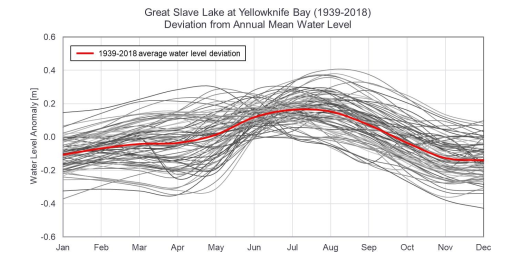
Figure 8.1 - Static water level anomalies on Great Slave Lake at Yellowknife (1939–2018).
Text version - Figure 8.1
Graph showing static water levels anomalies on Great Slave Lake between 1939 to 2018
The relative magnitude of long-term (e.g., decadal) and seasonal/annual variability should be considered when evaluating lake levels for the purpose of lakeshore flood hazard analysis.
Changes over decadal time scales may be caused by large-scale climate variability that influences regional and continental precipitation and evaporation patterns (e.g., El Niño-La Niña Southern Oscillation, North Atlantic Oscillation, etc.).
As an example, illustrating the different time scales relevant to lake water level variability, monthly (static) water levels on Lake Erie are shown in Figure 8.2 for the period 1918–2020. The lowest water levels occurred during the 1930s, and periods of high water levels have occurred nearly every decade since the 1950s. The seasonal water level range on Lake Erie is approximately 0.5 m and the long-term range is nearly 2 m.
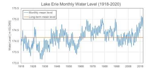
Figure 8.2 - Lake Erie long-term water level variations.
Text version - Figure 8.2
Graph showing Lake Erie long-term water level variations
8.1.2 Storm Surge
Storm surge is the temporary increase (or decrease) in the water level due to meteorological conditions. It may include:
- Wind set-up: The downwind increase in water level occurring as a result of shear stress exerted by the wind on the water surface.
- Barometric set-up: The increase in water level due to changes in atmospheric pressure during storm events.
The factors that primarily affect wind set-up are:
- Wind speed: Shear stress increases quadratically with wind speed.
- Water depth and shoreline configuration: Wind set-up is amplified in shallow water and enclosed bays.
- Fetch and duration: Wind blowing over larger distances for a longer duration produces more wind set-up.
- Lake surface roughness: The roughness of the air-lake interface (e.g., as determined by wave and/or ice conditions) influences momentum transfer and the resulting wind set-up.
- Ice: The presence of mobile ice floes can enhance air-water momentum transfer through increased surface roughness and form drag, amplifying wind set-up. Conversely, extensive or shorefast ice cover reduces (or eliminates) the effective fetch and suppresses or dissipates wind set-up.
Barometric set-up is a small component of storm surge on lakes and can be ignored when the pressure differential over the lake surface is less than a few millibars. This is usually the case for large non-convective storm systems passing over most lakes.
8.1.3 Seiche
Seiches are standing waves, caused by meteorological effects or other excitation mechanisms (e.g., earthquakes), which slosh back and forth within a lake. They can form after a storm surge, when water that was pushed to one end of the lake subsides.
Estimating seiche elevations is challenging because they depend on how close the excitation frequency (i.e., related to the passage of the storm surge) is to the natural oscillation frequency of the lake, which depends on the lake geometry and bathymetry, and the effects of frictional damping. Elongated lakes tend to be more prone to amplifications. In general, the potential for seiches should be evaluated if there is knowledge or evidence pointing to periodic (regular) water level oscillations on the order of minutes. Simplified methods for estimating the natural free-oscillation period of a closed basin (e.g., a lake) are provided in various engineering manuals (e.g., CIRIA et al., 2007; USACE, 2002). Estimates of seiche potential and heights may be derived from analysis of historical water level records or numerical modelling of lake hydrodynamics.
8.1.4 Wave Runup and Overtopping
The wave runup elevation is the maximum elevation of wave uprush on the shore above the still water level. It consists of:
- Wave set-up: The super-elevation of the mean water level at the shore due to wave breaking.
- Swash: The uprush and downrush of water on the shore, resulting in fluctuations about the wave set-up elevation.
Wave runup is a complex phenomenon that depends on the local water level, fetch, nearshore water depth, incident wave conditions (height, period, direction, breaking or non-breaking), and the nature of the beach or structure at the coast (e.g., slope, reflectivity, height, permeability, roughness) (FEMA, 2005).
When the wave runup elevation exceeds the crest elevation of a beach or coastal structure, water flows over the crest. This is referred to as “green water” overtopping. Overtopping flows can pose direct hazards to people and property or contribute to inland flooding.
Another form of wave overtopping can occur when waves break on the seaward face of a steep or vertical structure, causing splash droplets to be carried over the crest by their own momentum or wind (EurOtop, 2018). This is particularly a concern for cold climates where spray can freeze to buildings and other structures.
8.2 Data Requirements
8.2.1 Topographic and Bathymetric Data
Topographic LiDAR is available for many parts of Canada and can be obtained from provincial sources and/or NRCan (2021).
Bathymetric data may be available from the Canadian Hydrographic Service (CHS, 2021a) and provincial sources. Data may be provided as navigation charts, field sheets, and/or digital data (e.g., single or multibeam echosounder, nearshore bathymetric LiDAR, etc.). For storm surge and wave modelling applications, relatively low-resolution bathymetry may be adequate in deep areas or where gradients are gentle, whereas higher resolution bathymetry data may be required in shallow regions or areas with steep bathymetric gradients. Nearshore bathymetric surveying (e.g., echosounder) is often carried out for projects where existing data is limited or not available. Bathymetric LiDAR is becoming increasingly available but has limitations with respect to water depth and turbidity.
Care should be taken when integrating topographic and bathymetric datasets to ensure a consistent vertical reference and minimization of digital artifacts, potentially through verification with cross-shore transects.
8.2.2 Cross-Shore Transects
Cross-shore transects may be required for one-dimensional wave runup and overtopping analyses. They may be derived from high-resolution topographic-bathymetric digital elevation models or surveyed using a combination of water/vessel-based and land survey techniques. Calm conditions are required for surveying in the surf zone, as shallow water, waves, currents, and mobile sediments can create challenges and hazards for a survey team. In cases where high-resolution data exists (e.g., topographic and bathymetric LiDAR, or multibeam data), transects can be derived from the base data provided the interpolation is only over small distances and elevations.
Transects should be representative of the typical topography and bathymetry for a particular shoreline reach. In general, transects will be perpendicular to the local bathymetric contours and shoreline. Transects (and reaches) should be spaced closer together where there are physical changes in the shoreline.
8.2.3 Water Level Data
Water level data are available from the Canadian Hydrographic Service (CHS, 2021b), Water Survey of Canada (2023), and provincial sources (e.g., provincial ministry of environment or natural resources, hydro utilities, universities, etc.). Data are generally available at daily and hourly (or more frequent) sampling intervals. Monthly mean water levels are also available for the Great Lakes (Lake Superior, Lake Michigan-Huron, Lake St. Clair, Lake Erie, and Lake Ontario) from 1918 to present (CHS, 2021b). The water levels for each lake are averages based on a network of gauging stations in Canada and the United States.
In most cases, the study site will not have a long-term water level gauge. However, if data is available for other locations on the lake, static water levels may be derived from the nearby gauge(s). Short-term water level measurements (e.g., weeks to months) at the study site may be used to develop correlations to the long-term water level gauge(s) and estimate extreme storm surges at the study site (e.g., Rogers et al., 2010). Although these methods are generally quicker to apply and less costly than numerical modelling, they should be applied with care, especially over long distances, or along complex coastlines due to site-specific differences.
For many lakes, long-term water level measurements are not available. In these situations, the maximum recorded water level (if available), maximum regulated water level (e.g., reservoir operating licence), or historical high-water marks could be used in place of the regulatory static water level (e.g., 1% AEP static water level). Estimates of wind set-up should be added to the static water level estimates when determining AEP flood levels.
Where no documented information exists, local knowledge and field reconnaissance (e.g., erosion or scarping of the backshore, differing vegetation types, driftwood/debris lines) may provide evidence of past high-water levels.
8.2.4 Meteorological Data
Hourly meteorological measurements are available from Environment and Climate Change Canada (2021a) for more than 2,000 stations across the country. Wind speed, wind direction, air pressure, and air temperature are typically used to estimate storm surge and wave conditions. Most principal stations are equipped with a U2A anemometer, which takes one- minute or (since 1985) two-minute mean wind speeds at each observation (e.g., hourly) (ECCC, 2021c). Wind directions are recorded to the nearest 10 degrees, while those from older instruments are provided to 8 points on a compass. Wind speed and direction are greatly affected by the height of the anemometer above ground and the presence of hills, buildings, and trees. The standard exposure of the anemometer cups is 10 m above the ground surface.
Reanalysis datasets, such as NOAA’s Climate Forecast System Reanalysis (CFSR) (Saha et al., 2010), the European Centre for Medium-Range Weather Forecasts’ ERA5 Reanalysis (Copernicus Climate Change Service, 2017), and ECCC’s Regional Deterministic Reforecast System (RDRS) (Gasset et al., 2021), may be used to drive storm surge and wave models for large lakes (where spatially varying meteorological data is required). However, the limitations of these datasets for lake applications, including low spatial resolution, poor resolution of surface atmospheric fields at the land/water interface, and/or their parameterization or omission of important atmosphere-lake interaction processes, should be considered. Some local validation of reanalysis data using measured data should be performed, to characterize uncertainty, and identify any needs for bias correction.
The presence (or absence), concentration, mobility, and characteristics (e.g., surface roughness) of lake ice are important considerations for wave and storm surge generation and propagation, since they affect effective fetch lengths and air-sea momentum transfer. Ice data are available from the Canadian Ice Service (2021) and NOAA’s Great Lakes Environmental Research Laboratory (2021a).
8.2.5 Wave Data
Wave buoy data (and ancillary meteorological data) is available from Fisheries and Oceans Canada (DFO, 2021) for Great Slave Lake, Lake Winnipeg, Lake of the Woods, Lake Nipissing, Lake Simcoe, and the Laurentian Great Lakes. Archived wave buoy data is also available from NOAA’s global wave buoy database (NOAA, 2021b). Wave buoys are usually removed in the fall to avoid ice damage. As such, wave measurements for fall and winter storms are generally not available. Well-calibrated and validated numerical models may be used to augment or fill gaps in historical datasets, particularly if local or regional knowledge suggests that records may have missed significant events.
Most marine coastal and Great Lakes flood mapping studies rely on long-term (multi-decadal) hindcasts of offshore wave conditions. The hindcast wave models are driven using meteorological data from observation stations and/or reanalysis datasets and are calibrated to measured wave buoy and meteorological data. No publicly available wave hindcasts are available for Canadian lakes; however, the U.S. Army Corps of Engineers’ Wave Information Study (USACE, 2021) includes output points along the Ontario shoreline of the Great Lakes.
8.3 Meteorological Data Analysis
8.3.1 Storm Climatology
Wind data should be reviewed to identify the seasonal and directional distributions of extreme wind speeds as a prerequisite for determining extreme wind speeds for storm surge and wave modelling and analysis. Extreme wind speeds tend to occur more frequently in the fall and winter when lake levels are generally low and/or covered by ice. Often, but not always, the wind directions associated with the most extreme events will coincide with the longest fetch; however, correlation of directional extremes and fetch distances should be considered.
8.3.2 Adjustment of Wind Speeds
Wind speeds may need to be adjusted before they can be used to estimate storm surge and wave conditions. Standard techniques are described in Part II of the Coastal Engineering Manual (USACE, 2002) and may include:
- Anemometer elevation: Adjust wind speeds to 10 m above the ground surface.
- Averaging period: Adjust wind speeds from the observation averaging period (e.g., 2 minutes) to a time appropriate for storm surge and wave generation (this depends on the size of the lake, see USACE, 2002).
- Anemometer location: Adjust wind speeds measured over land to overwater conditions (if required, see USACE, 2002).
- Atmospheric boundary layer: Adjust wind speeds to account for thermal stability effects near the air-water interface. This is particularly important for fall storms, when the lake surface is warmer than the air and momentum transfers are enhanced.
8.4 Static Lake Level Analysis
Static water levels are water levels where the short-term fluctuations (caused by wind, waves, seiches, passing ships, etc.) have been removed by averaging over time. Typically, the averaging period will range from a few days to a month.
Weekly and/or monthly average lake levels may be available directly from data providers or calculated from daily, hourly, or more frequently sampled data (e.g., 5 minutes). Moving averages and more sophisticated filtering techniques (e.g., Gaussian, low-pass, etc.) are used to remove short-term fluctuations from the water level record. Static lake water levels may be determined for a single gauge or multiple gauge locations.
8.5 Storm Surge Analysis
Storm surge analysis involves the estimation of wind set-up using simplified methods, analysis of water level records, or hydrodynamic models. These approaches are described in the following subsections, with guidance on key considerations and the application of each method. The outcome of the analysis is an estimate of storm surge, which is combined with the static lake level to determine the AEP flood water levels.
8.5.1 Simplified Storm Surge Estimation Methods
The simplified methods typically involve the use of analytical models or empirical formulae to predict contributions by wind effects to water levels (e.g., methods provided in Chapter 4 of the Rock Manual (CIRIA et al., 2007)). These methods are generally appropriate for preliminary assessments, for sites where simplifying assumptions are valid (e.g., constant and homogeneous wind fields, no significant variation in water depth), or where high levels of uncertainty in the estimates can be tolerated. Simplified methods are usually adequate for smaller lakes.
The general procedure involves:
- Determine extreme wind speeds and directions using statistical methods (e.g., peaks- over-threshold analysis to estimate wind speeds for different AEPs).
- Estimate wind set-up at the downwind shoreline using analytical formulae for simplified cases (e.g., closed basin of constant depth).
- Estimate wind set-up at the study location using interpolation methods.
If measured water level data is available (at the study site or other locations on the lake), the analytical formula should be calibrated to historical storm surge events. Otherwise, the predicted storm surge values should be used with caution, and sensitivity analyses should be carried out to select appropriate (and representative) values for the wind drag coefficient, basin length, and water depth.
8.5.2 Analysis of Long-term Water Level Gauge Records
These approaches involve an analysis of gauge data to decompose total water level records into static water level and residual (assumed representative of storm surges) components. The resulting residual time series may be compared to historical wind data to establish correlations between wind events/directions, fetches, and storm surges; and to confirm or rule out the possibility of other processes contributing to residuals (e.g., seiches or tsunamis). Joint probability or statistical frequency analysis may be applied to the resulting time series data to assign probabilities to extreme storm surge events. Records with sampling intervals of 1 hour (or more frequent) are typically required to characterize storm surges; longer (e.g., daily) intervals between sampling may miss peak surge events. This type of analysis is only possible where long-term water level records exist for the site of interest.
An estimate of storm surge using gauge records is shown in Figure 8.3. In this example, the static water level and still water level were estimated by applying moving average filters with windows of 30 days and 1 hour, respectively, to water level data sampled at 5-minute intervals. The residual (an estimate of the storm surge) is the difference in elevation between the still water level and the static water level. Peaks-over-threshold analyses (e.g., Goda, 2010; CIRIA et al., 2007) should be used to determine extreme storm surges for the desired AEPs based on computed residuals.
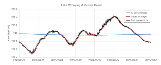
Figure 8.3 - Estimation of storm surge and static water levels from long-term water level gauge records.
Text version
Graph showing estimation of storm surge and static water levels from long-term water level gauge records.
8.5.3 Storm Surge Modelling
Numerical modelling predictions of storm surges generally involve the use of 2-D (depth- averaged) or 3-D hydrodynamic models that allow for prescription of temporally and spatially varying wind fields, pressure fields, and ice concentrations to generate storm surge predictions near the shore. Numerical modelling is generally appropriate or required:
- Where long-term records are not available.
- Where necessary to gain in-depth understanding of the spatial distribution of storm surges.
- To investigate hypothetical or future storm scenarios.
- To examine the effects of changes and development in the coastal zone on storm surges.
- To support analysis of flood-generating pathways (e.g., overtopping and erosion).
- To provide input to overland flood hazard modelling and mapping (optionally, nested or unstructured grid techniques may be used to integrate lake-wide storm surge and overland flood hazard modelling).
Different hydrodynamic modelling approaches may be taken depending on the size of the lake and/or overall risk levels. Guidance on setting up and applying storm surge models is provided in numerous documents (e.g., USACE, 2002; FEMA, 2016b; FEMA, 2014). For situations where higher levels of uncertainty can be tolerated (e.g., preliminary assessments, smaller lakes, etc.), the approach may involve:
- Determine extreme wind speeds and directions using statistical methods (e.g., peaks- over-threshold analysis to estimate wind speeds for different AEPs) or select discrete storm events to simulate in the model.
- Develop the hydrodynamic model mesh/grid using GIS data to define the model extents (shorelines) and bathymetric/topographic data to define the depths/elevations in the model.
- Simulate wind set-up on the lake for either:
- Steady-state wind conditions: constant and homogeneous wind fields.
- Discrete storm events: time-varying and homogeneous wind fields.
For situations where a higher level of certainty is required (e.g., medium to large lakes, significant exposure of lakeshore communities and/or valued assets, etc.), detailed hydrodynamic modelling may include the following in addition to the general procedure described above:
- Field acquisition of detailed bathymetry and topography near the study location.
- Refinement of the computational mesh/grid to capture important shoreline and bathymetric features.
- Use of time- and spatially varying reanalysis datasets (wind and air pressure data) to drive the models for the simulation of historical storm surge events.
- Use of time- and spatially varying ice cover datasets.
For all situations, historical gauge records should be used to calibrate and validate the hydrodynamic models to provide confidence in the model results and to quantify uncertainty. Where gauge records are sparse or absent, other sources of data for model calibration may include historical high-water mark surveys, debris line elevations, photographs, morphological evidence of high-water level marks (e.g., erosional scarps), or remotely sensed inundation outlines.
The key parameters for calibrating storm surge models for lakes are:
- Wind stress: This is typically parameterized using a drag coefficient that varies with the wind speed (USACE, 2002; FEMA, 2014; FEMA, 2016b). The drag coefficient may be adjusted to account for the effects of ice on wind-lake momentum transfer (Chapman et al., 2005, 2009; Joyce et al., 2019; Kim et al., 2021). Calibrated wind drag coefficients for lakes may be higher than typical values for marine coasts.
- Bed friction: Energy dissipation due to bottom friction is usually parameterized using a Manning or Chézy coefficient. Storm surges in shallow water will be more sensitive to the bed friction coefficient.
- Eddy viscosity: This is typically used to parameterize sub-grid turbulence. Some models use a simple constant eddy viscosity while others use a more complex formulation based on the velocity field and local grid size (e.g., Smagorinsky formulation).
- Computational mesh/grid resolution: Refinement of the model mesh/grid in key areas (e.g., shoals, bays, around islands, etc.) may improve the predictive ability of the model.
8.6 Wave Analysis
Wave analysis involves offshore wave generation, nearshore wave transformation, and wave- shore interaction. These processes can be estimated using simplified methods and/or numerical modelling techniques. The outcomes of the analyses are an estimate of wave runup elevations and/or overtopping discharges, which can then be used to delineate lakeshore flood hazards.
The general procedure for estimating wave hazards involves:
- Estimate offshore wave conditions.
- For small lakes or preliminary analysis: Use simplified wave estimation methods that relate fetch-limited wave conditions to wind speeds, fetch distances, and water depths.
- For large lakes or detailed analysis: Use 1-D or 2-D spectral wave models to simulate the development of wind-generated waves or acquire long-term (multi- decadal) wave hindcast data for offshore locations.
- Estimate nearshore wave conditions.
- For shallow nearshores: Use simplified methods to estimate depth-limited wave conditions (breaking waves). This approach may result in more conservative estimates compared to the methods below.
- For small lakes or preliminary analysis: Use simplified wave transformation methods that account for wave refraction, shoaling, and breaking due to local bathymetry or use 1-D spectral wave models.
- For large lakes or detailed analysis: Use 2-D spectral wave models to simulate wave refraction, shoaling, breaking, bottom friction, and other processes that may be important at the study site (e.g., wave-current interaction, etc.). The use of nested modelling approaches or unstructured meshes that provide higher resolution near the shoreline may allow for wave generation and wave transformation modelling to be combined in one step.
- Estimate wave runup elevations and/or overtopping discharges.
- For small lakes or preliminary analysis: Use empirical equations.
- For large lakes or detailed analysis: Use empirical equations, 1-D cross-shore wave models, or advanced numerical models capable of simulating swash zone processes.
- Estimate wave overtopping-induced hazards.
- For backshores with positive slopes (water flows back to the lake): Use empirical equations, or advanced numerical wave models to estimate water depths, velocities, and excursions.
- For backshores with negative slopes (water flows to topographic depressions): Use numerical hydrodynamic models to assess overland flood hazards driven by wave overtopping discharges.
8.7 Wave Generation
8.7.1 Simplified Wave Generation Methods
Simplified methods described in the Coastal Engineering Manual (USACE, 2002) and Rock Manual (CIRIA et al., 2007) may be used to estimate wind-generated waves. These methods are generally appropriate for preliminary assessments, for sites where simplifying assumptions are valid (e.g., constant and homogeneous wind fields, no significant variation in water depth), or where high levels of uncertainty in the estimates can be tolerated. The formulae relate the wind speed, fetch distance, duration, and water depth to a characteristic wave height and period.
CIRIA et al. (2007) recommends three methods for application on lakes and reservoirs with restricted fetches (Saville method, Donelan method, and Young and Verhagen method). For large lakes, the methods that were developed for open oceans are recommended (e.g., USACE, 2002; CIRIA et al., 2007). Wave heights and periods should be estimated using a variety of methods whenever simplified equations are used. If available, measured wave data (e.g., wave buoys, bottom-mounted wave instruments, etc.) should be used to verify wave estimates.
The general procedure to estimate wind-generated wave conditions involves:
- Define the lake characteristics.
- Measure fetch distances from the study site to the opposite lakeshore for points around a compass (e.g., in 10°, 15°, 22.5° increments).
- Estimate the average water depth for each fetch.
- Define the wind characteristics using one of these methods.
- Determine extreme wind speeds and directions using statistical methods (e.g., peaks-over-threshold analysis to estimate wind speeds for different AEPs).
- Prepare the wind data (e.g., gap filling, etc.) for simulating long-term wave hindcasts.
- Estimate wave conditions for wind speeds and various directional fetches using empirical equations. This will give one of these results:
- Wave heights and periods for the corresponding extreme wind speeds and directions.
- An estimate of wave conditions for the entire wind record, from which extreme wave conditions can be extracted.
8.7.2 Wave Generation Modelling
Wave generation modelling is the simulation of historical wave conditions, typically using wind data as driving input to the model. The modelling is carried out using consistent model physics and input datasets (e.g., meteorological reanalysis and ice cover datasets) to allow for the estimation of extreme value and operability statistics. Hindcast data is usually provided as a time series of wave parameters (e.g., height, period, direction, etc.) or spectral data. Output points are generally restricted to offshore (deep-water) locations where waves are not affected by water level variations and shallow-water processes.
The effort required to develop a multi-decadal wave hindcast is beyond the scope of most lakeshore flood mapping studies. Different approaches to develop extreme wave conditions include:
- Long-term simulation (multi-decadal) to include storm events.
- Simulation of discrete storm events including the temporal evolution of waves during the storm.
- Simulation of discrete storm events for the peak of the storm.
The modelling may be carried out using 1-D or 2-D spectral wave models that are capable of simulating wave growth from wind inputs, transfer of wave energy from high to low frequencies, and dissipation due to whitecapping. Historical wave buoy data should be used to verify wave model results when measured data is available.
Reporting should include a description of the model set-up, physical processes simulated by the model, and verification metrics.
8.8 Nearshore Wave Transformation
The nearshore is the shallow water region where waves interact with the lakebed (generally areas where the water depth is less than about one-half the wave length). In this region, wave crests will refract to align with the lakebed contours and waves will increase in height as they enter shallower water (shoaling). Waves may also lose energy (decrease in height) due to breaking and bottom friction, and change direction or height due to interaction with waves from other directions, currents, etc. Typically, 1-D and 2-D phase-averaged spectral wave models are used to simulate nearshore wave transformation processes. In some cases, simplified methods or advanced phase-resolving wave models may be appropriate for estimating nearshore wave conditions.
For lakeshore sites that are protected by islands, headlands, breakwaters, etc., it may be necessary to estimate wave diffraction around the obstacles. This is typically done using phase- resolving wave models (e.g., Boussinesq models), or spectral wave models (using a phase- decoupled refraction-diffraction approximation) when higher levels of uncertainty can be tolerated.
8.8.1 Depth-Limited Waves
In some situations, the nearshore wave conditions will be limited by the water depth. For shallow nearshores, it is helpful to estimate the breaking wave height as this may guide the level of effort in determining both the offshore and nearshore wave conditions. Methods for estimating depth-limited waves (breaking due to water depth) are provided in USACE (2002) and CIRIA et al. (2007).
8.8.2 Simplified Nearshore Wave Estimation Methods
Simplified methods described in USACE (2002), CIRIA et al. (2007), and Goda (2010) may be used to estimate nearshore wave conditions. These methods are generally appropriate for preliminary assessments, for sites where simplifying assumptions are valid (e.g., uniform slope, straight and parallel bottom contours), or where high levels of uncertainty in the estimates can be tolerated. The formulae estimate the change in wave height from the offshore to the nearshore due to wave refraction, shoaling, and breaking. For irregular bottom profiles, it is often more convenient to use a 1-D (or even 2-D) spectral wave model than to apply the simplified formulae. Simplified methods (e.g., USACE 2002) may be used to estimate wave diffraction for very simple geometries.
8.8.3 Nearshore Wave Transformation Modelling
Nearshore wave modelling is recommended for most lakeshore flood studies. 1-D and 2-D spectral wave models simulate all the important nearshore wave processes (e.g., shoaling, refraction, breaking, diffraction, etc.) and provide more reliable results than the simplified methods described above. Nearshore modelling is required for lakes with irregular bathymetry and/or complex shorelines (e.g., headlands, islands, etc.).
Phase-resolving wave models require more effort and expertise to apply and are often used for studies where wave diffraction and wave-structure interaction are important (e.g., wave agitation in harbours).
The use of nested modelling approaches or unstructured meshes that provide higher resolution near the shoreline may allow for wave generation and wave transformation modelling to be combined in one step. This is typically the approach that is taken when wave hindcast datasets are not available. For situations where the offshore wave conditions are developed independently, the nearshore wave modelling will involve the development of 1-D transects or a 2-D model grid/mesh for the nearshore region and propagation of the offshore wave conditions to the shore. The nearshore wave modelling should be carried out using water levels developed using desktop analyses or storm surge modelling.
The following approaches are used to simulate discrete storm events or transform the entire time series of offshore wave data to nearshore locations:
- Simulation of wave conditions for discrete storm events using coupled hydrodynamic and wave models to simulate the temporal evolution of waves and storm surge. This method involves running the models on the same computational grid/mesh and passing inputs and outputs between models (i.e., dynamic coupling). For lakes, it is usually adequate to run the wave model using the outputs from the storm surge model (i.e., offline coupling) rather than passing outputs back and forth. Very high-resolution models are required to resolve wave set-up at the shoreline due to the narrow surf zones on most lakes (FEMA, 2014).
- Same as above but simulating wave and storm surge conditions for only the peak of the storm. This approach is generally appropriate for small to medium lakes where steady- state conditions are likely to be achieved.
- Simulation of wave conditions for discrete storm events using a nearshore wave model and offshore waves as the boundary conditions. The model may be run using water levels from desktop analyses or storm surge modelling.
- Simulation of wave conditions for a matrix covering the full range of offshore wave height, period, direction, and water levels using a nearshore wave model. A time series of nearshore wave conditions is then created from the time series of offshore conditions by interpolating the model results over the four variables.
The key considerations for nearshore wave transformation modelling are:
- Bathymetry: Quality and resolution of bathymetric survey data; representation of bathymetry in the model (grid resolution, irregular features, etc.).
- Water levels: Nearshore processes are strongly influenced by the water depth.
- Physical processes: Careful review of important physical processes to be simulated in the model.
8.9 Wave Runup and Overtopping Analyses
Wave runup and overtopping can vary substantially along a shoreline due to differences in wave exposure, nearshore bathymetry, shoreline topography, and surface roughness. In most cases, the shoreline should be classified into reaches (where conditions are similar), and wave runup and overtopping estimated using one or more representative profiles for each reach.
Wave-shore interaction, including wave runup and overtopping, is a complex phenomenon that depends on the water level, wave conditions, bathymetric/topographic profile, and characteristics of the shore or coastal structures. Wave runup elevations (and overtopping discharges) fluctuate during a storm in response to the sequencing and interactions of individual waves and wave groups. By convention, the elevation exceeded by 2% of waves is used to characterize wave runup associated with a storm event. For most Canadian lakes, this corresponds to the elevation that would be exceeded by about 10–20 waves (e.g., wave periods between about 4–10 seconds) during the most intense hour of storm activity.
Empirical formulae and 1-D cross-shore models are typically used to estimate wave runup elevations and the properties of overtopping waves for flood mapping studies. Physical model experiments and advanced numerical models may be used when a higher level of certainty is required.
Empirical methods use a simplified representation of the physics of the wave runup and overtopping process to relate the response parameters (e.g., 2% runup elevation and mean overtopping discharges) to the key wave and structure parameters (EurOtop, 2018). Empirical coefficients and constants used in the formulae are derived from physical model testing or field measurements. As such, the formulae are prone to uncertainty and inaccuracy if used to extrapolate beyond the limits of parameters and conditions for which they were developed. It is recommended that they be used by experienced practitioners with knowledge of the origins, limitations, and applicability of the formulae (e.g., Murphy and Khaliq, 2017).
While empirical formulae have traditionally been used to estimate wave runup elevations, guidance in FEMA (2014) for flood mapping studies on the Great Lakes recommends the use of 1-D cross-shore models based on the non-linear shallow water equations for most shoreline conditions (except for very gently sloping, dissipative beaches). These models simulate many of the important surf zone processes, operate on a fine grid scale (e.g., 1-m grid spacing), and are well suited for modelling large numbers of profiles and storms. A benefit of 1-D modelling is that the shoreline profiles are used directly in the model, whereas empirical formulae require the user to derive geometric characteristics from the profiles. This can be quite subjective and should be done by experienced practitioners with knowledge of the formulae. The U.S. Army Corps of Engineers conducted a review of wave runup tools for flood hazard studies and recommended the use of the open-source CSHORE model (Kobayashi, 1997, 2009) due to its good predictive skill and ease of use (Melby, 2012).
The following methods are recommended for flood mapping studies on Canadian lakes:
- Steep shorelines and coastal structures: The EurOtop (2018) manual provides the most up-to-date guidance and calculation tools for evaluating wave runup and overtopping of dikes, revetments, and seawalls. The “design and assessment approach” formulae should be used for flood mapping studies (see e.g., FEMA, 2021).
- Complex profiles including beaches, steep shorelines, and coastal structures: 1-D cross- shore models based on the non-linear shallow water equations should be used for complex profiles, including most beaches (except very gently sloping, dissipative beaches), and steep shorelines and coastal structures that are outside the range of experimental conditions in the EurOtop (2018) manual.
- Simple beach profiles: The Coastal Engineering Manual (USACE, 2002) provides methods for evaluating wave runup on smooth planar slopes. These methods may be used for simple beach profiles or to verify 1-D model results. Note that empirical formulae developed for very gently sloping beaches, such as Stockdon et al. (2006), may underestimate wave runup for conditions typical on Canadian lakes.
8.9.1 Wave Overtopping-Induced Hazards
Wave overtopping occurs when the wave runup elevation exceeds the height of the natural or constructed barrier. Overtopping flows, splash, and spray can pose direct hazards to people and property or contribute to inland flooding.
Overtopping can become very severe when the still water level is near (or above) the elevation of the barrier. Hydrodynamic models may be required in this situation to simulate the overland flow of wave overtopping discharges.
The depth, velocity, and excursion of “green water” overtopping can be estimated using empirical formulae, 1-D cross-shore models, and advanced numerical wave models. For coastal flood mapping studies, the horizontal distance that an overtopping wave (or bore) will travel inland before it decays to a thin film is the primary concern. The high-velocity wave zone may also be mapped. This zone is usually very narrow, in the order of a few metres for lake shorelines, and is where the water depth and velocity can significantly damage infrastructure.
The general procedures for estimating wave overtopping-induced hazards are:
- Determine if overtopping occurs. Does the runup elevation exceed the height of the crest?
- If yes, proceed to Step 2.
- If no, use the runup elevation for mapping wave hazards.
- Estimate the mean overtopping rate and “excess runup” height (runup elevation minus crest elevation). Does the mean overtopping rate pose a hazard to people, vehicles, or property (see e.g., USACE, 2002; EurOtop, 2018)? Does the excess runup height exceed 1 m? Are there low backshore areas vulnerable to flooding/ponding?
- If yes to any, proceed to Step 3.
- If no to all, use a minimum distance of 5 m (measured from the crest) for mapping wave hazards.
- Evaluate the backshore topography. Is the plateau flat or sloping towards the lake?
- If yes, (flat or positive slope) use empirical equations or advanced numerical wave models to estimate water depths, velocities, and excursions.
- If no, (negative slope) use hydrodynamic models to assess overland flood hazards driven by wave overtopping discharges (e.g., flow to low areas and ponding). If required, high velocity wave overtopping zones may also be mapped using empirical equations or advanced numerical wave models.
A simplified procedure for estimating the horizontal excursion of overtopping waves is described in several guideline documents (e.g., Ontario Ministry of Natural Resources, 2001; FEMA, 2005; CIRIA et al., 2007). The method is based on a theoretical formulation by Cox and Machemehl (1986) for a bore of water propagating overland. This simplified method can be used in many situations or as a check if using more advanced approaches. The equations and definition sketch are shown in Figure 8.4.
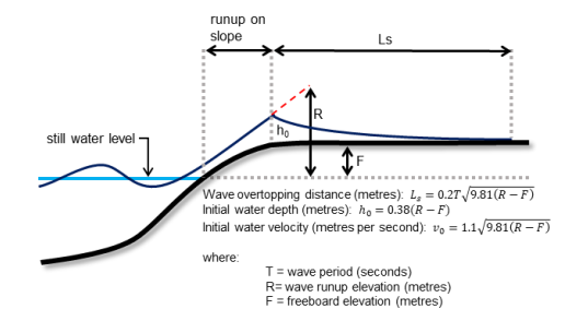
Figure 8.4 - Cox-Machemehl method for estimating wave overtopping-induced hazards.
Text version - Figure 8.4
Figure showing the Cox-Machemehl method for estimating wave overtopping-induced hazards.
8.10 Mapping Lakeshore Flood Hazards
Lakeshore flood hazard maps define areas that are directly inundated at the still water level and areas that are exposed to wave effects and other water-related hazards (e.g., wave spray, debris, ice, etc.). The maps may also define different hazard intensities (e.g., high velocity wave hazards). In some cases, lakeshore hazard maps will show flood and other natural shoreline hazards, such as erosion, slope instability, and dynamic beaches (not covered in this guide).
The horizontal limit of wave runup and overtopping should be estimated on a reach basis where wave and shoreline conditions are similar. It is recommended that several cross-shore transects be used for each reach because the estimated runup and overtopping values can vary due to differences such as the local water depth and shoreline slope.
On smaller lakes, estimated wave allowances are usually in the range of 5 m (or less), while estimates in the range of 10 m to 20 m are more common for larger lakes. Wave allowances should be reviewed (and possibly increased) for sites vulnerable to icing from wave spray, ice piling (ice accumulation), or debris impacts.
The lakeshore flood hazard limit for a given event is delineated in one of several ways depending on whether waves overtop the shoreline slope (see Figure 8.5):
- When no overtopping occurs, the flood hazard limit is mapped using the elevation contour corresponding to the wave runup elevation.
- When overtopping of a natural or constructed barrier with a flat or positive slope occurs, the flood hazard limit is mapped using the wave overtopping distance measured from the crest of the slope. Hazard mapping may also include delineation of the limits of tolerable mean wave overtopping discharges applicable to various uses (e.g., people, vehicles, structures, etc.) based on calculations or simulations.
- When overtopping of a natural or constructed barrier with negative slope occurs, or when a barrier is submerged, the flood hazard limit may extend far inland. The estimated overtopping rate and drainage features are used to identify areas subject to ponding and estimate the elevations of ponded water. Hydrodynamic models and wave models may be used to estimate the extents of overland flooding and wave effects.
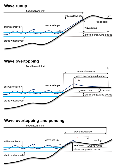
Figure 8.5 - Definition of lakeshore flood hazards for wave runup and overtopping.
Text version - Figure 8.5
Three separate figures illustrating wave runup, wave overtopping and wave overtopping and ponding.
8.11 Climate Change Considerations
Regional climate change information should be reviewed to evaluate potential impacts to static water levels, storm surge, and waves. As mentioned previously, static water levels are driven by hydrologic processes and future water levels will be affected by changes in:
- Precipitation patterns (e.g., magnitude and timing of extreme precipitation, winter rainfall, snowfall, etc.).
- Snowmelt (e.g., timing and volume of runoff, etc.).
- Evapotranspiration (e.g., changes due to temperature, ice cover on lakes, land use/land cover, etc.).
- Water use (e.g., withdrawals for irrigation, hydropower, etc.).
Climate change has the potential to affect storm surges and waves due to changes in:
- Static water levels (i.e., storm surges and wave heights are strongly influenced by the water depth).
- Storm systems (e.g., changes in wind speed, storm tracks, timing—e.g., storms occurring during periods of higher or lower water levels, etc.).
- Ice cover (e.g., changes in open-water season, winter storms, shorefast ice, etc.).
- Coastal geomorphology (e.g., changes to due lake level and storm variations).
Potential changes should be reviewed and addressed through numerical modelling or other approaches that consider a range of potential future conditions (e.g., different static water levels, ice-free winter conditions, etc.).
8.12 Lakeshore Flood Frequency Analysis
Lakeshore flood frequency analysis involves the estimation of static water levels, storm surges, and the joint probabilities of storm surges occurring at different static water levels. The general procedure for estimating extreme water levels involves the following steps:
- Convert from regulated to natural water levels where applicable.
- Determine the degree of seasonality for static water levels and storm surge. If it is significant (e.g., high static water levels during periods of low wind set-up or vice-versa), the data should be subdivided into seasons.
- Determine extreme static lake levels using the annual maximum (AM) method for the desired AEPs (annual or subdivided by season).
- Determine extreme storm surges using the peaks-over-threshold (POT) method for the desired AEPs (annual or subdivided by season).
- Determine extreme still water levels using the joint probability approach for the desired AEPs. The approach uses the static lake level and storm surge probability distributions as inputs.
8.12.1 Sample Size
The sample should be large enough to represent the local climate and meteorological mechanisms associated with extreme water levels, and waves and should not just cover the calm or stronger period of activity. Additionally, the data should be reviewed alongside nearby stations and other sources to identify data gaps to determine if extreme events were missed.
Changing conditions over time (e.g., decrease in lake ice) may mean that present-day conditions (e.g., winter storm surges) may be less frequently observed in the historical record. In these situations, it may be preferable to use a smaller sample size rather than the entire period of record (e.g., use most recent 40–50 years rather than 80 years of record).
The sample size duration should represent at least half of the extreme AEP being extrapolated (e.g., a sample of at least 50 years is recommended for estimating a 100-year return value, i.e., AEP of 1%). Extrapolating beyond these limits should be done with caution.
8.12.2 Stationarity
Most extreme value analysis methods used in practice rely on the assumption of stationarity, which may not be valid for areas that have experienced historical change (e.g., flow regulation) or impacts from climate change (e.g., changing lake ice conditions). Tests for trends, seasonality and stationarity are described in Hawkes et al. (2008). The removal of trends and non-stationarity are recommended prior to conducting extreme value analyses (e.g., Murphy and Khaliq, 2017).
8.12.3 Seasonal Analysis
The degree of seasonality should be determined for static water levels and storm surge. If it is significant, the extreme value analysis should be subdivided into seasons. For example, strong storms are often more frequent in the fall and winter when static lake levels are low. In many situations, ignoring seasonality (assuming high static water levels and strong winds could occur together) will result in overly conservative estimates of still water levels.
Subdividing the data further (e.g., by month) should also be done with caution, especially when the period of record is short. If the data is subdivided by month, it may be desirable to include data within two weeks of the start and end of the month to prevent over-segmentation (e.g., a storm that occurred on September 30 should be included in the monthly statistics for September and October).
8.12.4 Annual Maximum Method
The annual maximum (AM) method is typically used to estimate extreme static water levels. Static water levels are driven by hydrologic processes and typically peak during the summer. The AM method extracts the highest value for each year.
8.12.5 Peaks-Over-Threshold Method
The peaks-over-threshold (POT) method is often used to estimate extreme storm surges. Storm surges are driven by wind events and can happen at any time of the year, but they are more frequent in the fall and winter. The POT method selects events based on their magnitude rather than the calendar year in which they occurred. As such, some years may have more than one event while other years may have none. In general, the threshold should be selected to yield between 1 and 3 events per year.
Techniques such as minimum storm duration, inter-event duration, etc. should be used to ensure independent events are selected (e.g., Mazas and Hamm, 2011; Murphy and Khaliq 2017). In some cases, it may also be necessary to review and separate the storm events by directional sector, meteorological phenomena, seasonal analysis, or outlier events (e.g., hurricanes) (e.g., Mazas and Hamm, 2011; Murphy and Khaliq, 2017).
8.12.6 Joint Probability Analysis
The joint probability analysis method is used to estimate the probability of two or more dependent or independent events occurring simultaneously. Any joint probability analysis should begin with an exploratory analysis of the relationship between the variables of interest. The dependence between variables dictates the approach for the analysis. When analyzing two variables (e.g., storm surge and wave height), two limit cases exist. One limit is that the variables are perfectly correlated (i.e., collinear), the other limit is that the two variables are completely independent. When the relationship is near either one of these limits, simplifying assumptions may be made. However, when the relationship is somewhere between these two limits, as is often the case in natural phenomena, the qualified professional should identify a reasonable approach for pairing AEPs of dependent variables.
For large lakes, it may be safe to assume that static water levels and storm surges are independent because they are driven by different processes and occur on different time scales. Many different combinations of static water levels and storm surges could result in the same flood levels. For example, the 1% AEP flood level (still water level) could occur from a large surge at a typical static water level, or from a small surge at a very high static water level.
In this case of essentially independent events, a “design event” using N-year return storm surge with both N-year return wave heights and N-year return precipitation may result in an AEP that is much lower than 1/N years. However, when two events are assumed to be dependent, the simple combination of two N-year events is appropriate.
A simplified approach to estimating design events in the case of two independent events is as follows:
- Estimate static water levels and storm surges for discrete AEPs using univariate extreme value analyses (e.g., 50%, 20%, 10%, … 0.2% AEP).
- For a specified still water level AEP (e.g., 1% AEP), identify different combinations of static water level AEP and storm surge AEP that when multiplied together equal the specified still water AEP (e.g., 50% static and 2% surge, 20% static and 5% surge, 10% static and 10% surge, etc.).
- Identify the static water level and storm surge combination (sum) that yields the highest still water level for a given AEP.
A simple approach that assumes a limit case (either fully dependent or fully independent) may be appropriate when tolerance for uncertainty is high. However, usually in the natural world, reality is somewhere between full dependence and independence. Thus, in higher risk situations, substantially more complex approaches may be warranted. Many approaches exist and are not detailed in these guidelines. The qualified professional should apply the most appropriate analysis for the situation.
8.12.7 Joint Probability of Waves and Water Levels
For smaller lakes, it may more often be that storm surges and waves are strongly correlated (both being generated by wind events). In such cases, the selected AEP wave condition (e.g., 10% AEP) may be assumed to occur in combination with the selected AEP storm surge (e.g., 10% AEP). However, on larger lakes, the joint probability of storm surges and waves may need to be explicitly considered or analyzed (e.g., FEMA, 2014; CIRIA et al., 2007). In the absence of concurrent wave and water level records of sufficient length to establish correlations, or where low sensitivity to dependence does not justify the time and expense of a rigorous site-specific analysis, conservative assumptions (i.e., strong correlation) or simplified methods (e.g., Defra/EA, 2005) may be applied.
It should be noted that it is unlikely that the 1% AEP wave condition (and wind speed) will accompany the 1% AEP flood level. In practice, the 1% AEP flood level is usually some combination of static water level and storm surge where each is in the range of the 5–20% AEP (e.g., 5% AEP static water level with 20% AEP storm surge). Different combinations of static water levels and storm surge should be reviewed to determine appropriate wave conditions for wave runup and overtopping analyses.
8.12.8 Stochastic Methods (Monte Carlo Simulation)
This approach simulates a large number of historical or synthetic (hypothetical) storms to create a database to extract flood results (e.g., water levels, storm surge, waves, runup, etc.) and derive extreme value statistics. This approach avoids preselecting which combinations of static water level, storm surge, and wave conditions lead to extreme coastal flooding. The approach is more involved and should be considered for complex sites and projects that require a higher level of certainty (e.g., higher-risk locations). Additional details are provided in Melby et al. (2012) and Nadal-Caraballo et al. (2012).
8.13 Reporting Requirements
The report on lakeshore flooding should cover the extent of the study site, flood hazard- generating events considered, the mechanism(s) of flooding, approaches to flood hazard modelling and analysis, water level frequency analyses, and the analytical approaches taken to assess the design water levels under current and future climates. Section 10.0 covers the reporting requirements in detail, including data transfer and documentation.
8.14 Summary of Practices for Lakeshore Flooding
The methods described above should be used for lakeshore flooding, driven by elevated lake levels, storm surges, and wave effects. If river discharges are also a source of flood hazards, the potential for compound flooding events involving fluvial and lakeshore flooding should be assessed. Qualified reviewers not involved in the project should examine the analysis before the production of the final report.
9.0 Uncertainty in Flood Hazard Assessment
Characterizing, documenting, and managing uncertainty is a universal aspect of robust flood hazard assessments. The sources of uncertainty in the assessment of flood hazards are many: the measurements and observations of random natural phenomena may lead to inaccurate data; the models, their analytical procedures and empirical equations have inherent biases and imperfections; and the parameter values are based on observed random nature. The flood hazard delineation study should acknowledge these uncertainties, and where appropriate, quantify and address them.
Some approaches to address uncertainty are the uncertainty sensitivity index method (USIM); the first-order second-moment method; Monte Carlo simulation using multi-objective simulation method (MSM); assigning probability density functions (PDFs) to the parameters; or by other similar uncertainty quantification methods, depending upon the situation. For example, in estimating uncertainty using a Monte Carlo simulation model, there are several options, not only for the distribution (e.g., normal, log-normal, uniform, triangular, box) of the parameter, but also for the sampling from the distributions (e.g., random, quasi-random, and stratified).
Section 9.1 describes a method of quantifying uncertainties associated with the calculation procedures discussed in the above sections for flood hazard delineation analyses. Section 9.2 covers the uncertainty in climate change models, while Section 9.3 qualitatively elaborates on the uncertainties inherent in the assessment of flood hazards and how reports and regulators might handle the uncertainties. Finally, Section 9.4 provides a summary of uncertainty in flood hazard assessments.
9.1 Quantification of Uncertainty
A method to quantify the uncertainty inherent in the analysis and modelling procedures of the design flood events is described in Figure 9.1.
The first step is combining the study objective function for the analytical method used, whether flood frequency analyses, extension of data, hydrologic, and or hydraulic modelling. This provides criteria for the tolerance of the comparison of the simulated sequence with the observed series. Practitioners determine if a bias correction is required to improve the match and run the model again. Once the simulated sequences are sufficiently close to the observed, no further bias correction is necessary.
Next conduct a sensitivity analysis of the model’s output to each non-constant parameter to determine the relative impact of each parameter, by adjusting each parameter a set amount and comparing the results. Uncertainty quantification requires the summation of the products of the sensitivity of each parameter and the uncertainty of that parameter. This analysis is referred to as the first-order second-moment (FOSM) method (ISO/EIC, 2008). Another tool now available to quantify uncertainty uses the multi-method approach of the VARS-TOOL, (Razavi et al., 2019). For more rigorous quantification a more expensive, time-consuming Monte Carlo simulation with multiple model runs would be necessary.
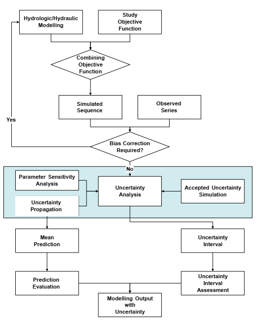
Figure 9.1 - Uncertainty of hydrologic and hydraulic modelling.
Text version - Figure 9.1
Figure describes a method to quantify the uncertainty inherent in the analysis and modelling procedures of the design flood events.
The range of model results would yield a mean prediction, such as the average value of the design events, with an uncertainty interval, expressed as confidence limits or minimum and maximum differences from the sensitivity analyses or the Monte Carlo simulations. Most probability distribution software generates confidence limits from the data used as input to the software. After assessing the prediction and the uncertainty interval against other methods and observed sequences, practitioners would be able to quantify the uncertainty of the hydrologic or hydraulic models in terms of the mean value and uncertainty interval.
9.2 Uncertainty in Climate Change Projections
Climate change uncertainty is the result of a cascade of uncertainties coming from various sources: emissions scenarios, climate models, downscaling and bias-correction methods, natural variability, statistical parameter estimation, and the applications methods that are being used to incorporate climate information as inputs. Regarding climate indicators for example, an uncertainty range of -5% to +200% is not uncommon when performing a sensitivity analysis on infrastructure design (Roy et al., 2017). Inter-comparison of applications methods, including hydrologic models, may be useful in ensuring that scenario-based impacts are assessed in a consistent manner, as previous studies have shown differences in hydrologic model representation of evaporation and snowmelt processes (Cohen et al., 2015).
The decision-making process can become much more complex in the context of these uncertainties. An ensemble approach, as described in Section 4.0, takes the results for meteorological factors influencing streamflow from a number of simulations of the future climate. If practitioners used a climate ensemble approach to the incorporation of climate change, the range of design flows and resultant flood hazard delineation results will quantify the uncertainty associated with the final determinations.
9.3 Uncertainty in Assessments of Flood Hazard Delineations
Changes in climate and land use can cause hydrologic, hydraulic, ice, and lakeshore flood assessments (and the flood hazard maps they support) to become less certain, and in some cases, obsolete. Planning of the initial study parameters to account for these potential changes maximizes the length of time that the final product will be relevant. Periodic review of modelling assumptions is particularly important where flood hazard maps form the basis for flood risk planning and regulation. Maintaining the data and models used in the hydrotechnical approach, along with periodic review and revisiting the policy, is a major component of adaptive management. Adaptive management is a powerful tool to counter uncertainty in the assessments of flood hazard delineations.
9.3.1 Planning for Potential Changes
Careful planning can avoid the need for frequent updates that increase cost and can create a “moving target” for municipal planning, growth, and development. A 30-year horizon for the flow assessment allows it to include future municipal planning of development and future climate change estimates.
As part of each flood hazard delineation study, practitioners should review the intended scope and use of the flood hazard delineation products in the context of ongoing and expected changes within the watershed and along the river corridor. Where possible, studies should identify an appropriate planning horizon for flood risk management and take into account any climate and land use changes that are expected within that planning horizon (e.g., sea-level rise, changes in precipitation, changes in rural land use, and urbanization of natural areas). Precautionary allowances may be appropriate in situations where uncertainty is high.
Consideration should also be given to planned flood mitigation works that may affect inundation extents, depths, or velocities. With careful planning for potential changes in land use, and in sea-level rise and hydrology due to climate change, a flood hazard delineation should allow for stable development.
9.3.2 Periodic Review
Many jurisdictions legislate periodic review of flood hazards. The flood risk directives of the European Union (European Parliament, 2007) legislate a periodic review of flood management plans. The United Kingdom (UK Environmental Agency, 2019) requires a review every six years, and FEMA must assess the need to revise flood mapping every five years (Department of Homeland Security, 2017). When the initial study has considered future land use changes and the uncertainty from potential changes from climate change, the longevity may be longer, unless a major event has transformed the watercourse (e.g., avulsion) or land use (e.g., wildfire). A flow, ice jam, or storm surge event larger than the historical record used in any FFA for a flood hazard delineation will modify the FFA resulting in updated estimates of the magnitudes of the AEP events. Such events should lead to a re-examination of the FFA. A review of the basic hydrology of the initial study will indicate whether updates are required so that map users can appropriately understand and manage risk. In addition, should the channel or infrastructure change from the initial study, a new hydraulic analysis will indicate whether risks of inundation have increased even if the hydrology remains essentially the same.
9.3.3 Adaptive Management Approach
An adaptive management approach addresses the uncertainties inherent in flood delineation by continually reassessing the inputs of the analytical models used and allowing for flexibility as new conditions or as improvements to the understanding of the driving processes arise. It leads to responses that anticipate the widest probable range of future scenarios that do not constrain future options and foresee changes by relevant monitoring of input data. In addition, adaptive management fully documents the data and procedures of the initial study. The jurisdiction should maintain the numerical models used during the analyses of the flood hazard delineation. When a review indicates that the land use, hydrology, sea-level rise, channel, or water body characteristics have differed significantly from the initial study, an update will be easier and less costly than starting without the other components archived.
Even a well-designed flood hazard delineation study will have a real or perceived shelf life, given land use changes, channel morphology changes, infrastructure modifications, and climate non-stationarities. Stewardship of the data and procedures entails thorough documentation and effective information management of the sources and numerical models. Along with regular periodic review to monitor the input data, the continual maintenance of data and models in a suitable archive may address the uncertainty of the relevance of past work, for a few years into the future. These stewardship practices are major components of adaptive management and are detailed in Section 10.0.
9.4 Summary of Uncertainty in Flood Hazard Assessment
Uncertainty in the flood hazard delineations is inevitable; however, practitioners should be able to acknowledge, quantify, and address the uncertainty. Probability distributions from frequency analyses should have associated confidence limits. Sensitivity analysis for model parameters should yield error bars for results of hydrologic and hydraulic models. Climate ensembles will generate a series of likely values for projected design flows. Regular review of flood hazard delineations and review after major precipitation events, or land use or geomorphic changes will keep delineations applicable to current hazards. An adaptive management approach facilitates the updating of flood hazard delineations.
10.0 Requirements for report format
This section is intended to assist provincial, territorial, and municipal agencies that are contracting flood hazard delineation studies. The overview section below provides, in general terms, the rationale and requirements for a report covering each technical aspect. A data stewardship section provides an explanation on how report documentation is an integral component of any flood hazard delineation study and its adaptive management, and Appendix A lists the requirements for technical reports on each aspect of a flood hazard delineation study.
The detailed requirements (Appendix A) may be included in a scope of work and should be edited by the agency to be specific to the project.
10.1 Overview
The technical documentation for the survey and base data, the hydrology, hydraulics, any ice- jam investigation, any wind and wave effects (lakeshore flooding), and maps must be produced in a manner that is consistent with this document. Technical documentation must be prepared in such a manner that the entire work can be recreated by any qualified practitioners without the need to refer to any other material. Further, practitioners are to be able to recognize and understand all the methods, approaches, and basic data, and rationale used for these methods, as ascertained by a competent reviewer. All reports must bear the professional/licence stamp and signature of the Project Manager/Project Engineer and reviewer. All reports must acknowledge the funding body/agency and the report covers must bear the agency logos alongside relevant municipality logo, if applicable. Maintaining the data and the models in a suitable archive facilitates the review process and any requirements for future updates. This adaptive management approach encourages periodic review of the flood hazard delineations to ensure that they remain relevant. Repeatability of results is critical in any adaptive management context. This requires that any agency should be able to replicate the results of a study based on the existing documentation, assumptions, and details provided by practitioners.
The technical documentation for each component of the flood hazard delineation should be prepared using the following format:
- Acknowledgements
- Introduction
- Objectives
- General description of watershed and study area
- History of flooding (newspaper, local inhabitants, police, churches, high-water marks, etc.)
- General background information
- Scope of work
- Criteria used for the report analysis (such as design floods, climate change scenario, land uses, channel stability, ice-jam and/or wind and wave (lakeshore) considerations)
- The quantification of uncertainty in the results
A survey and base data report or section should discus the following criteria:
- Data used in analyses and calibration work, including the reasons for the choice of data.
- Information, other than the most current, used in the analyses.
- Justification for the selected watershed parameters used in the study.
A design flood events report or section covering the hydrology analyses should cover the following criteria:
- The specific criteria used in the selection of the approach for determining the design flood events.
- The criteria used in any flood frequency analysis (FFA); reasons for choosing a particular statistical distribution.
- The hydrologic modelling parameters and choice of any model.
- Method used and assumptions made in the calculation of the effects of infrastructure that influences streamflow and water levels, such as culverts, bridges, breakwaters, stormwater management ponds, reservoirs, embankments, and dikes. Include method used and assumptions on lakes, tributaries, and land use impacts on flows.
- Method and assumptions for assessing climate change.
A hydraulics report or section should mention the following criteria:
- The rationale for the choice of the particular model used in the analysis.
- Criteria used in locating and defining the cross-sections or mesh used in hydraulic calculations on a reach-by-reach basis. Method used and assumptions made in the determination of the starting water surface elevations for hydraulic model.
- The specific criteria used to determine where the effective flow limits of the model domain are located and boundary conditions.
- Reasons for using the selected Manning's roughness and hydraulic loss coefficients in determining the design flood water surface profiles.
- Method used and assumptions made in the calculation of the effects of the bridges, culverts, crossings, and embankments on water surface profiles; selection of bridge routine and reasons for each crossing.
- Methods used and assumptions made in the determination of spill flows; effects on downstream flows and flood line, areas affected due to the spill.
An ice-jam report or section should include the assumptions made and methods used with respect to parameter estimation at various stages of hydrologic and hydraulic analysis if an ice- jam analysis was conducted.
Any coastal impact report or section should include the impacts of coastal water levels on the flood levels, where relevant, and the details of the analytical method chosen and how it was incorporated in the analyses, including the sources of input data.
More granular and specific details of what to include in each report are listed in Appendix A.
10.2 Data Stewardship
Exhaustive reports as detailed in Appendix A are an integral component of the stewardship of the data and procedures through their documentation and archiving of the input data, sources, and numerical models. Indigenous communities are stewards of their own data following the First Nations ownership, control, access, and possession (OCAP®) principles discussed in Section 3.5.2. Revisions require document control, dating, and explaining the reasons for the revision. The continual maintenance of data and models in a suitable archive, along with periodic review and monitoring of the hydrology, land use, channel morphology, and infrastructure, may address the uncertainty of the relevance of past flood hazard delineations, well into the future. The archiving and stewardship process must allow the replicability of results. Given the many subjective decision points available to the water resources professional, documentation of the previous decisions and data stewardship are critical to ensure results can be replicated.
11.0 Conclusion
This document provides guidance for specifying and conducting hydrologic and hydraulic analyses for flood hazard assessment in Canada. It is not intended to supersede other federal, provincial, territorial, or local legislation, regulations, bylaws, policies, program standards, or technical guidance. Publication of Version 2.0 of this document provides a basis for flood hazard assessment, incorporating the impacts of climate change and elaborating on uncertainty. Future updates are anticipated to expand the scope and detail of the document, as mentioned in the preface.
12.0 References
AAFC (2017). Agriculture and Agri-Food Canada Agroclimate Impact Recorder.
Alberta Environment and Parks (1993). Review of flood stage frequency estimates for the City of Fort McMurray. Report prepared for the Technical Committee, Canada-Alberta Flood Damage Reduction Program by Technical Services and Monitoring Division, Water Resources Services. Edmonton, Alberta.
Alberta Transportation (2001). Guidelines on Flood Frequency Analysis. Alberta Transportation, Civil Projects Branch. Edmonton, AB. 74pp.
Andres, D. D. (1999). The effects of freezing on the stability of a juxtaposed ice cover. River Ice Management with a Changing Climate: Dealing with Extreme Events. CGU HS Committee on River Ice Processes and the Environment. 10th Workshop on the Hydraulics of Ice Covered Rivers, Winnipeg, Manitoba, Canada
Andres, D. D. & Doyle, P. F. (1984). Analysis of break-up and ice jams on the Athabasca River at Fort McMurray, Alberta. Canadian Journal of Civil Engineering 11-3: 444-458.
Associate Committee on Hydrology (1989). Hydrology of floods in Canada – A guide to Planning and Design, Ed Watt, Chief Editor, National Research Council, Ottawa, Ontario
AutoDesk (2020). Infoworks 1-D and 2-D.
Beard, L. R. (1974). Flood Flow Frequency Techniques: Technical Report CRWR-1198, Center for Research in Water Resources, University of Texas at Austin
Beltaos, S. (1983). River ice jams: theory, case studies and applications. Journal of Hydrologic Engineering, ASCE, 109-10: 1338-1359.
Beltaos, S. (Ed.) (1995). River Ice Jams. Water Resources Publications. Littleton, CO.
Beltaos, S. (2012). Distributed function analysis of ice jam flood frequency. Cold Regions Science and Technology, 71: 1–10.
Beltaos, S. (2013a). Hydrodynamic characteristics and effects of river waves caused by ice jam releases. Cold Regions Science and Technology, 85: 42-55.
Beltaos, S. (2013b). Chapter 7. Freeze Up jamming and formation of ice cover. in: River Ice Formation. CGU-HS Committee on River Ice Processes and the Environment (CRIPE), Edmonton, pp 181-255.
Beltaos S. (2021). Assessing the Frequency of Floods in Ice-Covered Rivers under a Changing Climate: Review of Methodology. Geosciences, 11(12):514.
Beltaos, S., Ismail, S. & Burrell, B.C. (2003). Midwinter breakup and jamming on the upper Saint John River: a case study. Special Issue on River Ice Engineering, Canadian Journal of Civil Engineering, ISSN 1208-6029, NRC Research Press, National Research Council Canada, 30(1): 77-88.
Beltaos, S. & Prowse, T.D. (2009). River-ice hydrology in a shrinking cryosphere. Hydrological Processes 23: 122-144.
Bezak, N., Brilly, M., & Šraj, M. (2014). Comparison between the peaks-over-threshold method and the annual maximum method for flood frequency analysis. Hydrological Sciences Journal, 59 (5), 959–977.
Bruce, J.P. (1976). National Flood Damage Reduction Program, Canadian Water Resources Journal, 1(1): 5-14.
Brunner, G. W. (2016). HEC-RAS River analysis system user’s manual. Version 5.0. U.S. Army Corps of Engineers, Institute for Water Resources, Hydrologic Engineering Centre, Davis, California, USA.
Brunner, G., Savant, G., & Heath, R.E. (2020). Modeler Application Guidance for Steady vs Unsteady, and 1-D vs 2-D vs 3-D Hydraulic Modeling, U.S. Army Corps of Engineers, Hydrologic Engineering Center, TD-41, 114 pp.
Bush, E. & Lemmen, D. S. (Eds.) (2019). Canada’s Changing Climate Report; Government of Canada, Ottawa, ON. 444 p. Available at changingclimate.ca
Canadian Ice Service (2021). Nautical Charts and Services. Available at ice-glaces.ec.gc.ca
Carson, R., Beltaos, S., Groenevelt, J., Healy, D., She, Y., Malenchak, J., Morris, M. Saucet, J-P., Kolerski, T., & Shen, H. T. (2011). Comparative testing of numerical models of river ice jams. Canadian Journal of Civil Engineering, 38: 669-678
Chang, C., Ashenhurst,, F. Damaia, S. & Mann, W. (2002). Ontario Flow Assessment Techniques (OFAT), Hydraulic Information Management, Brebbia, C.A., & W.R. Blain (Eds.), WIT Press, Ashurst, Southampton, U.K., pp. 421-431.
Chapman, R. S., Kim, S. C., & Mark, D. J. (2009). Storm-induced water level prediction study for the Western Coast of Alaska. Draft Report to POA, U.S. Army Engineer Waterways Experiment Station, Vicksburg, MS.
Chapman, R. S., Mark, D., & Cialone, A. (2005). Regional tide and storm-induced water level prediction study for the West Coast Alaska. Draft Report to POA, U.S. Army Engineer Waterways Experiment Station, Vicksburg, MS.
Charron, I. (2014). A Guidebook on Climate Scenarios: Using Climate Information to Guide Adaptation Research and Decisions. Ouranos, 86p.
Chow, V. T. (1959). Open-Channel Hydraulics. McGraw-Hill, New York. CHS (2021a). Nautical Charts and Services. Available at www.charts.gc.ca
CHS (2021b). Tides, Currents, and Water Levels. Available at www.waterlevels.gc.ca
CIRIA, CUR, & CETMEF (2007). The Rock Manual: The use of rock in hydraulic engineering (2nd edition). C683, CIRIA, London.
Clay (2022). ‘We're still concerned': Brampton officials say more flooding possible in Churchville area over next few days. Brampton Guardian.
ClimateData.ca (2022). Topic 6: Intensity-Duration-Frequency (IDF) Curves Climate Data for a Resilient Canada.
Cohen, S., Koshida G. & Mortsch, L. (2015). Climate and water availability indicators: Challenges and a way forward. Part III – Future scenarios. Canadian Water Resources Journal / Revue canadienne des ressources hydriques, 40-2: 160-172.
Cohn, T. A., England, J. F., Berenbrock, C. E., Mason, R. R., Stedinger, J. R., & Lamontagne, J. R. (2013). A Generalized Grubbs-Beck Test Statistic for Detecting Multiple Potentially Influential Low Outliers in Flood Series. Water Resources Research. 49-8: 5047-5058.
Cohn, T. A., Lane, W. L., & Baier, W. G. (1997). An algorithm for computing moments-based flood quantile estimates when historical flood information is available. Water Resources Research 3-9: 2089- 2096.
Commission for Environmental Cooperation (2020). North American Land Change Monitoring System. Land use datasets.
Copernicus Climate Change Service (C3S) (2017). ERA5: Fifth generation of ECMWF atmospheric reanalyses of the global climate. Copernicus Climate Change Service Climate Data Store (CDS), Available at https://cds.climate.copernicus.eu/cdsapp#!/home
Coulson (1991). Manual of Operational Hydrology in British Columbia, British Columbia Ministry of Environment, Water Management Division, Hydrology Section 2nd Ed 238pp.
Coulson, C. H. & Obedkoff, W. (1998). British Columbia Streamflow Inventory. BC Ministry of Environment, Lands and Parks, Resources Inventory Branch, Water Inventory Section. 56pp.
Cox, J. C. & Machemehl, J., (1986). Overland Bore Propagation Due to an Overtopping Wave. Journal of Waterway, Port, Coastal and Ocean Engineering, Vol. 112, pp. 161–163.
Crutcher, H. L. (1975). A note on the possible misuse of the Kolmogorov-Smirnov Test. Journal of Applied Meteorology. 14: 1600-1603.
CSA (2019). CSA Plus 4013-2019: TECHNICAL GUIDE Development (PDF 456 kb), Interpretation and Use of Rainfall Intensity-Duration-Frequency (IDF) Information: Guideline for Canadian Water Resources Practitioners.
CSA (2021). Ordering RADARSAT-2 Data.
Cunderlik, J. M., Jourdain, V., Ouarda, T. B. M. J., & Bobée, B. (2007). Local Non-Stationary Flood- Duration-Frequency Modelling. Canadian Water Resources Journal / Revue canadienne des ressources hydriques, 32(1): 43-58.
Cunge, J. A., Holly, F. M., Verwey, A. (1980). Practical Aspects of Computational River Hydraulics. London: Pitman Publishing Limited.
Cunnane, C. (1973). A particular comparison of annual maxima and partial duration series methods of flood frequency prediction, Journal of Hydrology, 18(3-4): 257-271.
Das, A, & Lindenschmidt, E-K. (2021). Modelling climatic impacts on ice-jam floods: a review of current models, modelling capabilities, challenges, and future prospects. Environmental Reviews 29(3): 378-390.
Defra/EA (2005). Joint Probability: Dependence Mapping and Best Practice: Technical report on dependence mapping, R&D Technical Report FD2308/TR1 (PDF, 2.3 mb).
Deltares (2020). SOBEK and Delft3D.
Department of Homeland Security (2017). FEMA Needs to Improve Management of its Mapping Programs Office of Inspector General p.2.
DFO (2021). Marine Environmental Data Section Archive.
DHI (2017). MIKE Extreme Value Analysis Toolbox (PDF, 600 kb)
ECCC (formerly Environment Canada) (1976). Hydrologic and Hydraulic Procedures for Flood Plain Delineation. Water Planning and Management Branch, Inland Waters Directorate, Ottawa climate.weather.gc.ca
ECCC (2021a). Historical Climate Data. Available at climate.weather.gc.ca
ECCC (2021b). Intensity-Duration-Frequency Files (IDF).
ECCC (2021c). Technical documentation: Climate Normals.
El Adlouni, S. & Bobée, B. (2015). Hydrological Frequency Analysis Using HYFRAN-PLUS Software, User’s Guide available with the software DEMO
El Adlouni, S., Ouarda, T. B. M. J., Zhang, X., Roy, R., & Bobée, B. (2007). Generalized maximum likelihood estimators for the nonstationary generalized extreme value model. Water Resources Research. 43-3.
England, J. F. Jr., Cohn, T. A., Faber, B. A., Stedinger, J. R., Thomas Jr., W. O., Veilleux, A. G., Kiang, J. E., & Mason, R. R. (2017). Guidelines for Determining Flood Flow Frequency – Bulletin 17C: USGS Techniques and Methods (PDF, 897 kb) book 4, chap. B5. 244 p.
European Parliament (2007). Directive 2007/60/EC of the European Parliament and of the Council of 23 October 2007 on the assessment and management of flood risks, 8 pp.
EurOtop (2018). Manual on wave overtopping of sea defences and related structures., Van der Meer, J.W., Allsop, N.W.H., Bruce, T., De Rouck, J., Kortenhaus, A., Pullen, T., Schüttrumpf, H., Troch, P. & Zanuttigh, B., Available at www.overtopping-manual.com.
FEMA (2003). Appendix F: Guidance for Ice jam Analyses and Mapping Guidelines and Specifications for Flood Hazard Mapping Partners. Federal Emergency Management Agency, United States Government.
FEMA (2005). Final Draft Guidelines for Coastal Flood Hazard Analysis and Mapping for the Pacific Coast of the United States. Oakland, CA.
FEMA (2014). Great Lakes Coastal Guidelines. In: Guidelines and Standards for Flood Hazard Mapping Partners, Appendix D.3 Update. Washington, DC.
FEMA (2016b). Coastal Water Levels. Guidance Document 67.
FEMA (2021). Guidance for Flood Risk Analysis and Mapping: Coastal Wave Runup and Overtopping.
Fill, H.D. & Steiner, A.A. (2003). Estimating instantaneous peak flow from mean daily flow data, Journal of Hydrologic Engineering, 8:365–369.
First Nations Information Governance Centre (2022). The First Nations Principles of OCAP®
Fuller, W.E. (1914). Flood flows, Trans. ASCE 77: 564-617.
Gasset, N., Fortin, V., Dimitrijevic, M., Carrera, M., Bilodeau, B., Muncaster, R., Gaborit, É., Roy, G., Pentcheva, N., Bulat, M., Wang, X., Pavlovic, R., Lespinas, F., Khedhaouiria, D., & Mai, J. (2021). A 10 km North American precipitation and land-surface reanalysis based on the GEM atmospheric model, Hydrol. Earth Syst. Sci., 25, 4917–4945,
Gaur, A. and Simonovic, S. P. (2018). Future changes in flood hazards across Canada under a changing climate. Water 10, 1441: 1–21.
Gerard, R. & Karpuk, E. (1979). Probability analysis of historical flood data. Journal of the Hydrology Division, ASCE, 105(HY9): 1153-1165.
Goda, Y. (2010). Random seas and design of maritime structures (Vol. 33). World Scientific Publishing Company.
Han, G., Ma, Z., Zai, L., Greenan, B., & Thomson, R. (2016). Twenty-first century mean sea level rise scenarios for Canada. Canadian Technical Report of Hydrography and Ocean Sciences 313.
Hardison, C. (1974). Generalized Skew Coefficients of Annual Floods in the United States, Water Resources Research, v.10, no. 4, p. 745-752
Hawkes, P. J., Gonzalez-Marco, D., Sánchez-Arcilla, A. & Prinos, P. (2008). Best practice for the estimation of extremes: A review. Journal of Hydraulic Research, 46(S2), pp.324-332.
Helsel, D. R. and Hirsch, R. M. (2002). Statistical Methods in Water Resources Techniques of Water Resources Investigations, Book 4, chapter A3. USGS
Hessami, M., Gachon, P., Ouarda, T. B. M. J., and St-Hilaire, A. (2008). Automated Regression-based Statistical Downscaling Tool. Environmental Modelling & Software. 23. 813-834.
Horritt, M. S. & Bates, P. D. (2002). Evaluation of 1D and 2D Numerical Models for Predicting River Flood Inundation. Journal of Hydrology 268(1-4): 87-99.
Hosking, J. R. M., & Wallis, J. R. (1997). Regional Frequency Analysis. Cambridge University Press.
Hughes, D. A. & Smakhtin, V. (1996). “Daily flow time series patching or extension: a spatial interpolation approach based on flow duration curves.” Hydrological Sciences- Journal-des Sciences hydrologiques, 41-6.
Hunter, N.M., Bates, P.D., Neelz, S., Pender, G., Villeneuva, I., Wright, N.G., Liang, D., Falconer, R.A., Lin, B., Waller, S., & Crossley, A.J. (2008). Benchmarking 2D Hydraulic Models for Urban Flooding (PDF, 345 kb). Water Management 161 (WMI): 13-30.
Huokuna M., Morris, M., Baltaos, S., & Burrell, B. (2017). Ice in regulated rivers and reservoirs. CGU Conference HS Committee on River Ice Processes and the Environment 19th Workshop on the Hydraulics of Ice-Covered Rivers at: Whitehorse, Canada.
ISO/EIC (2008). ISO Guide 98-3: 1995 and 2008 Uncertainty in measurement.
James, T. S., Robin, C., Henton, J. A., & Craymor, M. (2021). Relative sea-level projections for Canada based on the IPCC Fifth Assessment Report and the NAD83v70VG national crustal velocity model (PDF, 566 kb). Geological Survey of Canada.
Jarrett & England (2002). Reliability of Paleostage Indicators for Paleoflood Studies. Ancient Floods, Modern Hazards: Principles and Applications of Paleoflood Hydrology. American Geophysical Union
Jasek, M. (2003). Ice jam release surges, ice runs, and breaking fronts: field measurements, physical descriptions, and research needs. Canadian Journal of Civil Engineering, 30-1: 113 – 127.
Joyce, B. R., Pringle, W. J., Wirasaet, D., Westerink, J. J., Van DerWesthuysen, A. J., Grumbine, R., & Feyen, J. (2019). High resolution modeling of western Alaskan tides and storm surge under varying sea ice conditions. Ocean Model. 2019, 141, 101421.
Kim, J., Murphy, E., Nistor, I., Ferguson, S., & Provan, M. (2021). Numerical Analysis of Storm Surges on Canada’s Western Arctic Coastline. Journal of Marine Science and Engineering, 9(3), p.326.
Khaliq, M.N. (2017). Flood Frequency Analysis: Review of Selected Software Tools, NRC Technical Report – UNCLASSIFIED: OCRE-TR-2017-003, Document Version 1.2
Khaliq, M.N. (2019). An Inventory of Methods of Estimating Climate Change-informed Design Water Levels for Floodplain Mapping, National Research Council of Canada: Ocean, Coastal and River Engineering Technical Report no. NRC-OCRE-2019-TR-011.
Kobayashi, N. (1997). Wave runup and overtopping on beaches and coastal structures. Research Report No. CACR-97-09. Center for Applied Coastal Research, University of Delaware.
Kobayashi, N. (2009). Documentation of Cross-Shore Numerical Model CSHORE. Research Report No. CACR-09-06, Center for Applied Coastal Research, University of Delaware.
Kovachis, N., Burrell, B. C., Huokuna, M., Beltaos, S., Turcotte, B., & Jasek, M. (2017). Ice jam flood delineation: Challenges and research needs, Canadian Water Resources Journal / Revue canadienne des ressources hydriques, 42-3: 258-268
Leclerc, M., Doyon, B., Heniche, M., Secretan, Y., Lapointe, M., Driscoll, S., Marion, J. & Boudreau, P. (1998). Simulation hydrodynamique et analyse morphodynamique de la rivière Montmorency en crue dans le secteur des Îlets. Rapport de recherche (R522). INRS-Eau, Québec.
Lemmen, D. S., Warren, F. J., James, T. S., & Mercer Clarke, C.S.L. (Eds.) (2016). Canada’s Marine Coasts in a Changing Climate; Government of Canada, Ottawa, ON, 274p.
Limerinos, J. T. (1970). Determination of the Manning Coefficient from Measured Bed Roughness in Natural Channels. Geological Survey Water Supply Paper 1898-B.
Lindenschmidt, K-E., Das, A., Rokaya, P., & Chu, T. (2016). Ice jam flood risk assessment and mapping. Hydrological. Processes, 30: 3754–3769
Lindenschmidt, K., Huokuna, M., Burrell B. C., & Beltaos, S. (2018). Lessons learned from past ice jam floods concerning the challenges of flood mapping, International Journal of River Basin Management, vol.16-4: 457-468
López, J. & Francés, F. (2013). Non-stationary flood frequency analysis in continental Spanish rivers, using climate and reservoir indices as external covariates, Hydrology and Earth System Sciences, 17: 3189-3203.
Luettich, Jr. & Westerink (2016). ADCIRC: A (Parallel) Advanced Circulation Model for Oceanic, Coastal and Estuarine Waters. Available at adcirc.org
Mazas, F., & Hamm, L. (2011). A multi-distribution approach to POT methods for determining extreme wave heights. Coastal Engineering, 58(5), pp.385-394.
MDA Ltd. (formerly MacDonald, Dettwiler and Associates Geospatial Services) (2021). RADARSAT-2.
Melby, J. A. (2012). Runup Prediction for Flood Hazard Assessment. U.S. Army Corps of Engineers, TR- XX-12
Melby, J. A., Nadal-Caraballo, N. C., & Ebersole, B. A. et al. (2012). Lake Michigan: Analysis of Waves and Water Levels, U.S. Army Corps of Engineers, TR-XX-12
Ministers Responsible for Emergency Management (2017). An Emergency Management Framework for Canada, Third Edition (PDF, 4.50 mb).
Moin, S. M. A. & Shaw, M. A. (1985). Regional Flood Frequency Analysis for Ontario Streams: Volume I, Single Station Analysis and Index Method. Inland Waters Directorate, Environment Canada, Burlington.
Moin, S. M. A. & Shaw. M.A. (1986). Regional Flood Frequency Analysis for Ontario Streams: Volume 2, Multiple Regression Method. Inland Waters Directorate, Environment Canada, Burlington
Murphy, E. & Khaliq, M. N. (2017). Input to Canadian National Guideline for Flood Hazard Mapping: Coasts and Lakes. Technical Report (National Research Council of Canada. Ocean, Coastal and River Engineering), no. OCRE-TR-2017-005.
Murphy, E., Lyle, T., Wiebe, J., Hund, S., Davies, M., & Williamson, D. (2020). Coastal Flood Risk Assessment Guidelines for Building and Infrastructure Design: Supporting Flood Resilience on Canada’s Coasts.
Nadal-Caraballo, N. C., Melby, J. A., & Ebersole, B. A., (2012). Lake Michigan: Storm Sampling and Statistical Analysis Approach. U.S. Army Corps of Engineers, TR-XX-12
Nayak, P.C., Sudheer, K.P., Rangan, D.M. & Ramasastri, K.S. (2004). A neuro-fuzzy computing technique for modeling hydrological time series, Journal of Hydrology, 291: 52-66.
NDMP (2021). National Disaster Mitigation Program (NDMP).
NOAA (2017). mPING Reporting: Crowdsourcing Weather Reports. Available at mping.nssl.noaa.gov
NOAA (2021a). Great Lakes Environmental Research Laboratory. Available at glerl.noaa.gov NOAA (2021b). National Data Buoy Center. Available at ndbc.noaa.gov
NRCan (2017). Report a Felt Earthquake (PDF, 432 kb).
NRCan (2018). Case Studies on Climate Change in Floodplain Mapping (Volume 1) (PDF, 654 kb).
NRCan (2019). National Hydrographic Network.
NRCan (2021). High Resolution Digital Elevation Model (HRDEM) - CanElevation Series.
NRCan & PSC (2018). Federal airborne LiDAR data acquisition guideline.
NRCan & PSC (2019). Federal geomatics guidelines for flood mapping.
NSERC (2020). Floodnet Regional Freqency Analysis (RFA). Available from GitHub at NSERC Floodnet- Research Outcomes-Tools
Ontario Ministry of Natural Resources (1982). HYDSTAT Computer Program for Univariate and Multi- variate Statistical Applications. Conservation Authorities and Water Management Branch.
Ontario Ministry of Natural Resources (1989). Great Lakes System Flood Levels and Water Related Hazards. Conservation Authorities and Water Management Branch.
Ontario Ministry of Natural Resources (2001). Great Lakes - St. Lawrence River System and Large Inland Lakes. Technical Guide for Flooding, Erosion and Dynamic Beaches. Watershed Science Centre, ISBN 0-9688196-1-3
Pariset, E., Hausser, R., & Gagnon, A., (1966). Formation of ice covers and ice jams in rivers, Journal of the Hydraulics Division, American Society of Civil Engineers, November 1966. physical descriptions, and research needs. Canadian Journal Civil Engineering, 30: 13-127.
PCIC (2021). Statistically Downscaled Climate Scenarios.
Pender, G. (2006). Briefing: Introducing Flood Risk Management Research Consortium. Proceedings of the Institution of Civil Engineers, Water Management, 159 (WM1): 3-8.
Pilon, P. J. & Harvey, K. D. (1993). Consolidated Frequency Analysis (CFA) DOS version available at Institute for Watershed Science – Software
Rajulapati, C., Tesemma, Z., Shook, K. Papalexiou, S., & Pomeroy, J. W. (2020). Climate Change in Canadian Floodplain Mapping Assessments Centre for Hydrology Report No. 17 (PDF, 589 kb)
Razavi, S., Sheikholeslami, R., Gupta, H. V., & Haghnegahdar, A. (2019). VARS-TOOL: A toolbox for comprehensive, efficient, and robust sensitivity and uncertainty analysis. Environmental Modelling and Software 112: 95-117.
Razmi, A., Golian, S., & Zahmatkesh, Z. (2017). Non-Stationary Frequency Analysis of Extreme Water Level: Application of Annual Maximum Series and Peak-over Threshold Approaches. Water Resources Management 31: 2065–2083.
Rogers, J., Hamer, B., Brampton, A., Challinor, S., Glennerster, M., Brenton, P., & Bradbury, A. (2010).
Beach Management Manual (second edition). CIRIA C685, London.
Roy, P., Fournier, É., & Huard, D. (2017). Standardization Guidance for Weather Data, Climate Information and Climate Change Projections. Montreal, Ouranos. 52 pp. + Appendixes.
Rokaya, P., Budhathoki, S., & Lindenschmidt, K.-E. (2018). Trends in the timing and magnitude of ice-jam floods in Canada. Scientific Reports. 8(1): 5834.
Saha, S., Moorthi, S., Pan, H. L., Wu, X., Wang, J., Nadiga, S., Tripp, P., Kistler, R., Woollen, J., Behringer, D., & Liu, H. (2010). The NCEP climate forecast system reanalysis. Bulletin of the American Meteorological Society, 91(8), 1015-1058.
Sangal, B.P. (1981). A Practical Method for Estimating Peak from Mean Daily Flows with Application to Streams in Ontario, Technical Bulletin No. 122, National Hydrology Research Institute, Inland Waters Directorate, Ottawa.
She, Y. T. & Hicks, F. (2005). Incorporating ice effects in ice jam release surge models. CGU HS Committee on River Ice Processes and the Environment. 13th Workshop on the Hydraulics of Ice Covered Rivers, Hanover, NH, pp. 470-484.
Shen, H. T. (2010). Mathematical modeling of river ice processes. Cold Regions Science and Technology, 62(1), 3-13.
Stockdon, H. F., Holman, R. A., Howd, P. A., & Sallenger, A. H. (2006). Empirical parameterization of setup, swash, and runup. Coastal Engineering 53, Elsevier, 573-588.
Strathcona Regional District (2021). Tsunami Resources – Northwest Vancouver Island Tsunami Mapping.
TELEMAC- MASCARET (2021). Telemac v.8 p2.
TUFLOW (2020). Flood, Urban Stormwater & Coastal Simulation Software.
UK Environmental Agency (2019). Guidance - Flood risk management plans (FRMPs): responsibilities.
USACE (2002). Coastal Engineering Manual. Engineer Manual 1110-2-1100, U.S. Army Corps of Engineers, Washington, D.C. (in 6 volumes).
USACE (2019). Statistical Software Package. HEC-SSP.
USACE (2021). HEC-RAS v.6.
USGS (2017). Verified Roughness Characteristics of Natural Channels.
USGS (2019). Guidelines for Determining Flood Flow Frequency Bulletin 17C. U.S. Department of the Interior; U.S. Geological Survey. Reston, Virginia. Draft: May 2019. Accessed 29 September 2021.
Vogel, R.M. (2017). Stochastic watershed models for hydrologic risk management, Water Security, Volume 1, July, pages 28-35.
Warren, F. J. & Lemmen, D. S. (2014). Canada in a Changing Climate: Sector Perspectives on Impacts and Adaptation. Government of Canada, Ottawa.
Wasko, C., Westra, S., Nathan, R., Orr, H. G., Villarini, G., Villabos Herrera, R., & Fowler, H. J., (2021). Incorporating climate change in flood estimation guidance. Philosophical Transactions of the Royal Society A 379: 20190548.
Water Survey of Canada (2023). Water Level and Flow. Available at www.wateroffice.ec.gc.ca Wilby, R. L., Dawson, C. W., & Barrow, E. M. (2002). SDSM – a Decision Support Tool for the Assessment of Regional Climate Change Impacts. Environmental Modelling and Software 17: 147-59.
WMO (2009). Manual on estimation of Probable Maximum Precipitation (PMP), ISBN 978-926-3101045- 9, WMO No. 1045, 291 pp.
WMO (2011). Manual on Flood Forecasting and Warning WMO-No. 1072. 2011 Edition.
WMO (2021). The Atlas of Mortality and Economic Losses from Weather, Climate and Water Extremes (1970–2019).
Zaerpour, M., Papalexiou, S. M., & Nazemi, A. (2021). Informing Stochastic Streamflow Generation by Large-Scale Climate Indices at Single and Multiple Sites. Advances in Water Resources: 156.
13.0 Bibliography
Adams, B. J. & Howard, C. D. D. (1986). Design Storm Pathology, Canadian Water Resources Journal, 11:3, 49-55, DOI: 10.4296/cwrj1103049
Bishop, C. T., & Donelan, M. A. (1989). Wave prediction models. Elsevier Oceanography Series (Vol. 49, pp. 75-105). Elsevier.
British Columbia Ministry of Environment (2009). Manual of British Columbia Hydrometric Standards. Prepared by the Science and Information Branch for the Resources Information Standards Committee, Version 1.0.
Brunner, G. W. (2022). HEC-RAS, River Analysis System, HEC-RAS User's Manual, Version 6.2 the Hydrologic Engineering Center (HEC), Davis, California 721 pp.
DHI (2021). MIKE+, MIKE FLOOD, MIKE21/3. Available at www.mikepoweredbydhi.com
Donelan, M. A. (1980). Similarity theory applied to the forecasting of wave heights, periods, and directions. Proceedings of the Canadian Coastal Conferences, p. 47-61, National Research Council, Ottawa.
EGBC (2017). Flood Mapping in British Columbia.
FEMA (2016a). Coastal Flood Frequency and Extreme Value Analysis. Guidance Document 76. FEMA (2020). Hydraulics: Two-Dimensional Analysis Guidance for Flood Risk Analysis and Mapping.
Fernandes, R. A., Bariciak, T., Prévost, C., Yao, H., Field, T., McConnell, C., Luce, J. and Metcalfe, R. (2019). Method for measurement of snow depth using time-lapse photography (PDF, 4.3 kb). Geomatics Canada open file 47, NRCan.
Fernandes R. A., Prevost, C., Canisius, F., Leblanc, S.G., Maloley, M., Oakes, S., Holman, K., & Knudby, A. (2018). Monitoring snow depth change across a range of landscapes with ephemeral snowpacks using structure from motion applied to lightweight unmanned aerial vehicle videos. The Cryosphere, 12: 3535– 3550.
Hendrick, A. R. & Marshall, H.-P. (2014). Automated snow depth measurements in avalanche terrain using time lapse photograph, Proceedings of the International Snow Science Workshop, Banff, 836-842.
Hughes, S. A. (1993). Physical Models and Laboratory Techniques in Coastal Engineering. Advanced Series on Ocean Engineering, Vol. 7. World Scientific.
Hydraulic modelling: best practice (model approach) Updated (2021).
INRS-ETE (2008). HyFran available from Water Resources Publications (INRS-ETE)
Intergovernmental Oceanographic Commission (2016). IOC Manuals and Guides No. 14 – Manual on Sea Level Measurement and Interpretation [online]
Khaliq, M. N. & Attar, A. (2017). Assessment of Canadian floodplain mapping and supporting datasets for codes and standards, Technical Report (National Research Council of Canada. Ocean, Coastal and River Engineering), no. OCRE-TR-2017-026, 111 pp.
Khaliq, M.N & Piche, S. (2017). 2D Hydrodynamic Models for Floodplain Mapping: Review of Selected Modelling Packages Technical Report No. OCRE-TR-2017-004, Document Version 1.2
Klemeš, V. (1987). Hydrological and engineering relevance of Flood Frequency Analysis. in: Singh V.P. (Ed.) Hydrologic Frequency Modeling. Reidel, Dordrecht. pp. 1-18.
NRCan (2015). Risk-based land-use guide: safe use of land based on hazard risk assessment. Geological Survey of Canada Open File 7772.
NRCan (2017). Way forward for risk assessment tools in Canada. Geological Survey of Canada Open File 8255.
Oakes, S., Fernandes, R. A., & Canisius, F. (2016). Protocol for photographic survey of snow depth stakes in Support of CCMEO Snow Depth from UAV Activities, CCRS Open File 28, 9pp
Ontario Provincial Mapping Unit (2017). User Guide for Ontario Flow Assessment Tool (OFAT). Ontario Ministry of Natural Resources and Forestry, Corporate Management and Information Division, Mapping and Information Resources Branch, Provincial Mapping Unit. 79pp.
Parajka, J., Haas, P., Kirnbauer, R., Jansa, J., & Blöschl, G. (2012). Potential of time â‘lapse photography of snow for hydrological purposes at the small catchment scale. Hydrological Processes. vol. 26- 22:3327– 3337.
Partnership for Water Sustainability (2021). Qualhymo Energy.
Pirazzini, R., Leppaneen, L., Picard, G., Lopez-Moreno, J. I., Marty, C., Macelloni, G., Kontu, A., von Lerber, A., Tanis, C. M., Schneebeli, M., de Rosnay, P., & Arslan, A. N. (2018). European in-situ snow measurements: practices and purposes. Sensors 2018, vol. 18-7 2016.
Québec MELCCC (2021). Water Level and Flow Rates.
Smith, C. D., Yang, D., Ross, A., & Barr, A. (2018). The Environment and Climate Change Canada solid precipitation intercomparison data from Bratt’s Lake and Caribous Creek, Saskatchewan, Earth System Science Data Discussions, 11:1-17.
USACE (2021). Wave Information Study. Available at wis.usace.army.mil
Walker, J., Murphy, E., Ciardulli, F., & Hamm, L. (2014). On the reliance on modelled wave data in the Arabian gulf for coastal and port engineering design. Coastal Engineering Proceedings, 1(34), p.28.
Appendix A: Requirements for Technical Reports
Appendix A lists the requirements for technical reports on each aspect of a flood hazard delineation study. The detailed requirements listed here may be included in a scope of work and should be edited by the agency to be specific to the project.
Part A: Survey and Base Data
- Discussion
- Field survey of bathymetry of channel, topography of flood hazard area, hydraulic and flood control structures, benchmarks, and highwater marks
- Method of collection and list of all field equipment used—name and version
- Datum, epoch, geoid
- High-water mark data (date, location, quality)
- Source of LiDAR, orthophotography, aerial imagery
- Source of bathymetry
- Source, availability, and location of hydrometric data (streamflow, water level, drainage area above gauge)
- Source, availability, and location of meteorological data (precipitation as rain or snow, temperatures, frost-free days, onset of melt, statistical properties)
- Source and availability of land use and soil data
- Historical data on ice jams (dates, location of jams, extent of flooding, etc.)
- Historical data on floods (dates, location, extent of flooding, etc.)
- Conclusions and Recommendations
- List of technical persons with qualifications that worked on the project
- Professional/licence stamp and signature of the Land Surveyor/Project Manager
- List of all software used—name and version
- Limitations (including disclaimers)
- References
Part B: Open Water Hydrology Assessment
- Summary
- Background information
- Previous hydrologic studies
- Open water flood history (dates, discharge magnitude)
- Inspection of the streamflow and meteorological stations and records
- Methodology used in determining watershed parameters
- Factors (lakes, reservoirs, land use, etc.) influencing runoff
- River crossings (bridges, embankments) with significant storage effect
- Rationale for methods used to determine and verify design flows for existing and future conditions
- Assessment of geohazards (e.g., debris floods, channel switching risk)
- Methodology for the Hydrologic Analysis
- Flood frequency analysis (FFA) option
- Choice of annual maximum (AM) instantaneous discharge or peaks-over-threshold (POT) selection method
- Conversion of regulated flows to natural conditions (naturalized)
- Statistical tests on the data samples prior to frequency analyses for independence, randomness, and homogeneity
- If any separation of peak events required, eventual recombination technique
- How study is dealing with non-stationary records
- Extension of streamflow records
- Transfer of location
- Choice of single-station FFA or RFFA
- Choice of frequency distribution amongst all evaluated, method of fitting, and distribution parameters for each distribution evaluated
- Graphical and numerical results for flood quantiles and confidence limits
- Source of regional hydrology used as basis for an FFA
- Any regression coefficients and primary and secondary equations for flood quantiles
- Any allowances for natural and human-caused changes that have been applied to account for issues, such as differing land use or future development
- Conversion to regulated conditions under probable reservoir operating procedures
- Any generation of synthetic hydrographs for design peaks
- Comparison of results with analysis by other methods, previous estimates, or recorded events
- Uncertainty of results
- Hydrologic model option
- Computer program(s) used and their limitations
- Routing techniques used
- Any upstream input to the model
- Data (observed hydrographs, rainfall amounts, spatial and temporal distributions of rainfall, antecedent moisture conditions, temperatures, other meteorological parameters, soil infiltration parameters, etc.) used in calibration
- Sensitivity analysis
- Calibration of model parameters
- Justification of the values of the calibrated parameters
- Validation of the model
- Results of the model
- Comparison of results with analysis by other methods, previous estimates, or recorded events
- Uncertainty of results
- Climate and land use change considerations
- Climate scenarios and models selected
- Sources of land use changes and extent and nature of change
- Downscaling method of climate model used
- Verification of hydrologic model(s) used
- Data (observed and projected precipitation amounts, spatial and temporal distributions of precipitation, observed and projected temperatures, other meteorological parameters, soil infiltration parameters, etc.) used
- Uncertainty analysis
- Sensitivity analysis
- Bias correction including the values of the calibrated and validated parameters
- Results of the model
- Comparison of results with analysis by other methods
- Uncertainty of results
- Flood frequency analysis (FFA) option
- Conclusions and Recommendations
- Magnitude of design flows for existing and future conditions
- Uncertainty values associated with design flows
- List of technical persons with qualifications that worked on the project
- Professional/licence stamp and signature of the Project Manager/Project Engineer
- List of all software used—name and version
- Limitations (including disclaimers)
- Recommendations for future study, including future planning horizon, necessitating next flood hazard delineation study
- References to the other current reports associated with the study, previous reports, and reports on the hydrologic techniques used
Part C: Hydraulics
- Summary
- Background information
- Previous hydraulic analysis
- Flood mechanisms of study
- Associated survey and base data report
- Source of observed water level profiles
- Methodologies and Assumptions
- Channel and flood hazard area characteristics
- Approach for dikes
- Geomorphic stability
- Ice-jam considerations
- Computer Program(s) Used for Hydraulic Analysis
- Hydraulic Modelling
- Hydraulic control points
- Starting water surface elevation and boundary conditions
- Channel slope profile
- Selection of bridge routines
- Effects of river crossings and tributaries
- Sensitivity analysis results
- Locations with more impact
- Range of perturbation
- Verification of model parameters
- Data used in calibration and validation
- Roughness and loss coefficient values for various recorded high flows
- Roughness and loss coefficient values for design flood
- Water surface profiles of design flows
- Flood levels determined by reservoir routing analysis, as necessary
- Flood levels determined by dam break analysis, as necessary
- Flood levels and velocities based on 1-D or 2-D modelling
- Manual flood extent modifications
- Flood-prone areas
- Urban
- Rural, agricultural
- Spill areas
- Natural/constructed
- Volume of spill flow
- Velocities of spill
- Impact on downstream flows and flood levels
- Extent, depth, and velocity of flooding due to the spill
- Hydraulic control points
- Uncertainty Range of the Hydraulic Results
- Conclusions and Recommendations
- Extent, depth, velocity, probability, and uncertainty of design flooding
- List of technical persons with qualifications that worked on the project
- Professional/licence stamp and signature of the Project Manager/Project Engineer
- List of all software used—name and version
- Limitations (including disclaimers)
- Recommendations for future study, including future planning horizon, necessitating next flood hazard delineation study
- References to the other current reports associated with the study, previous reports, and reports on the hydraulic techniques used
Part D: Ice Jam (where relevant)
- Summary
- Background
- Information on previous ice analyses
- Mechanisms of past flooding caused by ice
- Associated survey and base data report
- Methodologies and assumptions
- Stage-frequency analysis of historic high-water levels related to ice jams, OR
- Synthetic stage frequency analysis assumptions, parameters, and results
- Hydraulic ice analysis: stage-discharge relationships under ice, roughness coefficients, and other parameters
- Computer program(s) used for ice analysis
- Uncertainties of results
- How climate change will likely impact ice jams on the study site
- Background
- Flood Frequency Analysis (FFA) of Ice-Affected Water Levels
- Choice of annual maximum (AM) or peaks-over-threshold (POT) selection method
- Conversion of regulated water levels to natural conditions
- Statistical tests on the data samples prior to frequency analyses for independence, randomness, and homogeneity
- If any separation of peak events required, eventual recombination technique
- How study is dealing with non-stationary records
- Consideration of non-systematic conception threshold water levels
- Choice of single-station FFA, RFFA, or synthetic FFA
- Choice of frequency distribution amongst all evaluated, method of fitting, and distribution parameters for each distribution evaluated
- Graphical and numerical results for flood quantiles and confidence limits
- Any regression coefficients and primary and secondary equations for flood quantiles of synthetic FFA
- Any allowances for natural and human-caused changes that have been applied to account for issues, such as differing land use or future development
- Conversion to regulated conditions under probable reservoir operating procedures
- Comparison of results with analysis by other methods, previous estimates, or recorded events
- Uncertainty of results
- Stage Discharge Curves Under Ice
- Choice of observed events used to generate curves
- Fitting of observed events to selected curves
- Conversion of EPA stages from FFA to EPA flows
- Hydraulic Modelling
- Hydraulic control points
- Starting water surface elevation and boundary conditions
- Selection of bridge routines
- Effects of river crossings and tributaries
- Ice parameters
- Roughness coefficient of top ice
- Jam coefficients
- Sensitivity analysis results
- Locations with more impact
- Range of perturbation
- Verification model parameters
- Data used in calibration and validation
- Roughness of and loss coefficient values for various recorded high ice-impacted flows
- Roughness and loss coefficient values for design flood
- Water surface profiles of design flows
- Flood levels determined by reservoir routing analysis, as necessary
- Flood levels determined by dam break analysis, as necessary
- Flood levels and velocities based on 1-D or 2-D modelling
- Flood-prone areas
- Urban
- Rural, agricultural
- Spill areas
- Natural/constructed
- Volume of spill flow
- Velocities of spill
- Impact on downstream flows and flood levels
- Extent, depth, and velocity of flooding due to the spill
- Uncertainty range of the hydraulic results
- Conclusions and Recommendations
- Design water levels, extent of flooding, velocities, and probabilities of ice-jam-influenced events
- Uncertainties associated with the ice-jam analyses
- Ice-jam flood hazard delineation
- List of technical persons with qualifications that worked on approach to ice analysis for the project
- Professional/licence stamp and signature of the Project Engineer/Project Manager
- List of all software used—name and version
- Recommendations for future study, including future planning horizon, necessitating next flood hazard delineation study
- Expectations under climate change
- Limitations (including disclaimers)
- References to the other current reports associated with the study, previous reports, and reports on the hydrologic and hydraulic techniques used.
Part F: Coastal Effects (where relevant)
- Summary
- Background
- Information on previous coastal analyses
- Mechanisms of past coastal flooding
- Associated Survey and Base Data Report
- Methodologies and Assumptions
- Storm surge assumptions, approach, data, and results
- Wave runup assumptions, approach, data, and results
- Justification for selected rate of sea-level rise, if applicable
- Joint probability methods and results
- Computer program(s) used in analysis
- Conclusions and Recommendations
- Design water levels, extent of flooding, velocities, and probabilities of coastal flood hazard delineation
- Uncertainties in the Coastal Flood Hazard Delineations
- List of technical persons with qualifications that worked on approach to the coastal analysis for the project
- Professional/licence stamp and signature of the Project Engineer/Project Manager
- List of all software used—name and version
- Recommendations for future study, including future planning horizon, necessitating next flood hazard delineation study
- Expectations of climate change impacts
- Limitations (including disclaimers)
- References to the other current reports associated with the study, previous reports, and reports on the hydrologic, hydraulic, and hydrodynamic techniques used
Part G: Maps in Appendices
- A large-scale topographic map in digital format showing:
- Elevation contours and point elevations of the flood hazard area, channel, and coast
- Extent of the study
- A small-scale topographic map in digital format showing:
- Watershed and sub-watershed boundaries
- Meteorological stations
- Hydrometric stations, extending to region used in any regional flood frequency analyses
- Land cover in the watershed (existing and future conditions)
- Soil types in the watershed
- Model cross-sections and/or mesh area of hydraulic model
- Observed water surface profiles at high flows
- Observed hydrographs, used to generate design hydrographs
- Water surface profile(s) of design flows(s) indicating depths, velocities, and extent of flooding
- Past locations of flooding and/or ice jam
- Other relevant data maps or diagrams
- Historical Aerial Imagery Analysis
Part H: Diagrams in Appendices
- Hydrologic model option
- Schematic diagram of the model
- Observed and simulated hydrographs in the calibration and validation analyses
- Hydraulics
- FFA option
- Probability curves of single-station or regional analysis versus plotted data
- Confidence limits
- Ice jam (where relevant)
- Stage-discharge relationship as a curve
- Other relevant data diagrams
- Data sheets of bridge and other hydraulic structures
- Plots of cross-sections and/or maps of DTM and bathymetry showing grid and mesh nodes
Part I: Tables in Appendices
- Hydrologic, meteorological, and hydrometric data
- Source
- Location, ID number, name
- Years collected
- Land cover and soil infiltration rates (hydrologic model option)
- Other relevant to study parameters
- FFA option
- Results of the frequency analysis, quantiles, and confidence limits
- Any transfer and correlation equations used in tabular form
- Any regression coefficients and primary and secondary equations for flood quantiles in tabular form
- Hydrologic model option
- Parameter data used in the model
- Meteorological data used
- Results of the sensitivity analysis of the parameters
- Data periods used in the calibration and validation steps
- Calibration and validation results
- Calculated and calibrated watershed parameters for existing and future conditions
- Comparison of flows by different methods for various return-period flow events
- Magnitude of design flows for existing and future conditions at various points of interest along the watercourse
- Uncertainty values associated with design flows
- Other tables of interest in the hydrologic analysis
- Hydraulic modelling results
- Hydraulic observed flow extents, velocities, and water levels at critical locations
- Results of sensitivity analysis
- Comparison of calibration and validation results with observed values
- Roughness and loss coefficient values for design flows
- Design flow extents, velocities, and water levels at critical locations
- Any relevant tables of data or results of the analysis
- Ice jam (where relevant)
- Details of past ice-jam-related flooding: dates, location of jams, extent of flooding, etc.
- Stage-frequency table
- Details of past coastal flooding: dates, location, extent of flooding, etc.
Part J: Other Appendices
- Open water assessment
- Input data and computer output of any FFA
- A large-scale topographic map of the watershed showing the sub-watersheds, overland flow, and channel lengths used in any time of concentration calculations, location of valley cross-sections, structures with significant storage
- Calculations of various watershed parameters (weighted slope, time of concentration, time to peak, recession constant, curve numbers etc.), rainfall reduction factors, storage- outflow relationships, regression and correlation analyses
- Input data and output for sensitivity analyses of any hydrologic model analysis
- Input data and output of the calibration and validation analysis of a model analysis
- Input data and summary output of any hydrologic model analysis
- RCM output used in estimating effects of climate change
- Uncertainty calculations
- Hydraulics
- Flood level calculations based on reservoir routing analysis for structures with significant upstream storage, where applicable
- Input data and output for the sensitivity analyses
- Input data and output of the final calibration and validation runs
- Input data and summary output of the hydraulic calculations
- All calculations for spill area analysis
- Input data and output of any dam break analysis
- Photographs of all structures
- Photographs of flood hazard area at representative reaches
- Photographs of high-water marks
- Other relevant information
Page details
- Date modified: