
Federal Flood Damage Estimation Guidelines for Buildings and Infrastructure
Version 1.0, 2021
Natural Resources Canada, General Information Product 124e
Natural Resources Canada, Public Safety Canada.
© His Majesty the King in Right of Canada, as represented by the Minister of Natural Resources, 2021.
For information regarding reproduction rights, contact Natural Resources Canada at copyright-droitdauteur@nrcan-rncan.gc.ca.
Table of Contents
- 1.0 Introduction and purpose
- 2.0 Note on terminology
- 3.0 General practices
- 4.0 Range of flood hazards and factors affecting damage
- 5.0 Types of flood damage
- 6.0 Tools for estimating damage
- 7.0 Stage-damage curves
- 8.0 Future adjustments and regional indexing
- 9.0 Case studies
- 10.0 References
- Appendix 1 – Breakdown of Flood Damage Calculation Steps
- Appendix 2 – Causes of Coastal Flooding
- Appendix 3 - Velocity Stage-Damage Curves for Buildings
- Appendix 4 – Damage Reductions Resulting from Contingency Measures
- Appendix 5 – Willingness-to-Pay Studies
- Appendix 6– Business Disruption and Residential Displacement Estimation Methods
- Appendix 7 – Costs Associated with Traffic Delays
- Appendix 8 – Flood Damage Assessment Tools
- Appendix 9 – Summary of Database Issues and Considerations
- Appendix 10 – Data Capture Forms – residential
- Appendix 11 – Data Capture Forms – non- residential
- Appendix 12 – Stage Damage Curves and Values - Residential*
- Appendix 13 – Stage Damage Curves and values - Non-Residential*
- Appendix 14 – Sample Content and Prices
- Appendix 15 – Review of Building Classification Schemes and Photographic Examples of Building Classes
- Appendix 16 – Residential Property External Damages
- Appendix 17 – Summary of Non- Residential Classes and Salvage of Contents
- Appendix 18 – Damages Suffered by Multi-Level Below-Grade Parkades
- Appendix 19 – Estimating Damages to Crops, Livestock, and Barns and Outbuildings
- Appendix 20 – Case study, damages to unique strutures: Stampede Park
- Appendix 21 – Uncertainty Associated with Structural Classification Schemes and Stage-Damage Curve Development
- Appendix 22 – Available Measures of Price and Spending Change
- Appendix 23 – Method for Updating Residential Content Damages Currency
List of abbreviations and acronyms
- AAD
- Average Annual Damages
- AEP
- Annual Exceedance Probability
- BCA
- Benefit-Cost Analysis
- BCP
- Business Continuity Planning
- BE
- Bare Earth
- CAD
- Canadian Dollars
- CBO
- Community Based Operations
- CEA
- Cost-Effectiveness Analysis
- CFDEP
- Comparative Flood Damage Estimation Program
- CME
- Contents Moved and Evacuated
- CPI
- Consumer Price Index
- CSVR
- Content to Structural Value Ratio
- DALY
- Disability Adjusted Life Years
- DEFRA
- Department for Environment Food and Rural Affairs
- DEM
- Digital Elevation Model
- EAD
- Expected Annual Damages
- EPA
- Environmental Protection Agency
- FDDBMS
- Flood Damage Database Management System
- FDO
- Flood Defence Operations
- FEMA
- Federal Emergency Management Agency
- FIA
- Federal Insurance Administration
- GDP
- Gross Domestic Product
- GIS
- Geographic Information System
- HAZUS-MH
- HAZUS Multi-Hazard
- HEC-FDA
- Hydrologic Engineering Center Flood Damage Reduction Analysis
- IPCC
- Intergovernmental Panel on Climate Change
- LiDAR
- Light Detection and Ranging
- LIRA
- Land and Infrastructure Resiliency Assessment
- MCA
- Multi-Criteria Analysis
- NDMP
- National Disaster Mitigation Program
- NOAA
- National Oceanic and Atmospheric Administration
- NRCan
- Natural Resources Canada
- PFDAT
- Provincial Flood Damage Assessment Tool
- QGIS
- Quantum GIS
- QRA
- Quantitative Risk Assessment
- RCP
- Representative Concentration Pathway
- RFDAM
- Rapid Flood Damage Assessment Model
- SHS
- Survey of Household Spending
- TBL
- Triple Bottom Line
- USACE
- U.S. Army Corps of Engineers
- USDA
- United States Department of Agriculture
- WCM
- Watercourse Capacity Maintenance
- WDR
- Warning Dependent Resistance
- WHO
- World Health Organization
- WTP
- Willingness To Pay
1.0 Introduction and purpose
This document is part of the Federal Flood Mapping Guidelines Series. These guidelines aim to provide advice to support the management of flood risks and their consequences to communities.
Since the late 1960s, a number of studies have been undertaken across the country and methodologies developed to assess flood damages within flood-affected communities, in order to quantify flood related damages, evaluate the cost-effectiveness of various flood mitigation projects and understand the vulnerability of people to flooding.
The following guidelines have been developed by the Government of Canada to establish a standardized approach for estimating damages to buildings and other infrastructure resulting from flooding and the development of flood stage-damage functions, incorporating international and national (provincial/ territorial/ regional) best practices where appropriate. Thus, this document, Federal Flood Damage Estimation Guidelines for Buildings and Infrastructure Version 1.0 is intended to provide a summary of the current practices used by qualified professionals in Canadian jurisdictions and to provide recommended practices for qualified professionals to estimate flood damage, primarily due to riverine flooding.
This document provides technical guidance and serves as a resource for engineers, scientists, insurers and municipal planners involved in flood damage estimation. In addition, this document describes a range of flooding hazards which can influence damages incurred as a result of flooding. The specific objectives of this document are to:
- Describe the range of flooding hazards and the factors affecting flood damage
- Describe different methods available for estimating damage resulting from flooding - primarily riverine
- Provide guidance on how to develop and use stage-damage curves as well as considerations on their use, accuracy and limitations
- Provide guidance for future adjustments and regional indexing of stage-damage curves
The scope of this document is limited to estimating damage, resulting from flooding, or prior to a flood event as part of a risk assessment. Refer to other documents in the series for guidance on other components of flood risk management in Canada.
2.0 Note on terminology
All Federal Flood Mapping Guidelines Series documents will apply the following definitions, based on the Emergency Management Framework for Canada (Ministers Responsible for Emergency Management, 2017) and NDMP (NDMP, 2021) literature. It is recognized that provinces and territories may define these terms differently, and these definitions are not intended to be prescriptive outside the context of the Federal Flood Mapping Guidelines Series documents.
Flooding: The temporary inundation by water of normally dry land.
Flood Mapping: The delineation of a flood on a base map. This typically takes the form of flood lines on a map that show the area that will be covered by water, or the elevation that water would reach during a specified flood event. The data shown on the maps, may also include flow velocities, depth, other risk parameters, and vulnerabilities.
Hazard: A potentially damaging physical event, phenomenon, or human activity that may cause the loss of life or injury, property damage, social and economic disruption, or environmental degradation.
Risk: The consequence of a specific hazard, expressed in terms of likelihood, and based on considerations of vulnerability and exposure.
Flood maps are used for several different purposes, including identifying hazards and risks, land use planning, emergency planning and response, and public awareness and communication. Under the broad definition of ‘flood map’, different types of geospatial, hydraulic, and hydrologic information can be presented to meet specific assessment requirements. For consistency, four main types of flood maps are defined here.
For the purposes of this document, the following definitions also apply:
Contents Damage: refers to damages to moveable contents within a structure
Depth-Damage Curve: see Stage-Damage
Design Flood: A specific flood magnitude that is used for delineating flood hazard areas.
Direct Damages: are those that occur immediately and can be directly attributed to flood inundation. Direct damages include damage to public infrastructure and private property.
First Floor Height: height of first floor above grade (Figure 6)
Grade: the highest elevation of the property which can be established using a DEM derived from LiDAR, from ground level surveys, or detailed topographic maps (Figure 6)
Indirect Damages: occur as a result of direct flood impacts but they are more difficult to quantify, examples include: reduced economic activity, individual financial hardships, adverse impacts on the social well-being of a community, and disruptive impacts
Intangible Damages: damages that are more difficult to assess monetarily such as emotional stress, illness, or loss-of-life
Resilience: strategies that focus on reducing impacts from flooding through prevention and preparedness
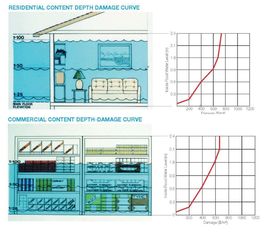
Stage-Damage: stage-damage and depth-damage are interchangeable terms which describe a one-dimensional mathematical relationship between the depth of water above or below the first floor of a building and the amount of damage that can be attributed due to that level of water (Figure 7). They typically represent the average damage of a group of buildings with similar properties due to flooding in a given community.
Empirical Stage-Damage vs Synthetic Stage-Damage: Empirical models use a data-driven approach, relying on actual damage datasets from past events in order to link building vulnerability to the record of damage data of the flood event. Synthetic curves are generated based on a conceptual approach and expert knowledge, hypothesizing and making assumptions about the potential damage, related to specific components of the building (McGrath et al. 2019).
Absolute vs Relative: absolute economic loss (in terms of currency) or relative loss (percentage of the estimated replacement value of property) of a buildings’ structure and contents. Most Canadian stage-damage curves are constructed using absolute value while in the U.S. the relative approach is most common.
Structure Damage: refers to damage to a building and the building components that are not taken when an individual moves, e.g.: furnace, hot-water heater, wall-to-wall carpeting. (IBI Group & Golder Associates, 2015)
Tangible Damages: damages to which a dollar value may be assigned.
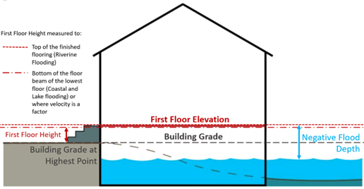
Figure 6: Building measurements used in determining flood depth
Text version
Figure of a house showing the building measurements used in determining flood depth
(source: IBI Group, 2015)
Figure 7: Example of Residential and Commercial stage-damage curves for contents
Text version
Figure showing an example of residential and commercial stage-damage curves for contents.
3.0 General practices
Practices in this document are included in each report section in tabular format. A summary of the general practices is included as Table 1, with additional information in Appendix 1.
| Number | General Practices |
|---|---|
| 1 | Flood Scenario and Depth Simulation. Refer to Federal Hydrologic and Hydraulic Procedures for Flood Hazard Delineation for details to develop a flood depth grid |
| 2 | Working with local community, assemble inventory of features that could be impacted, including buildings, infrastructure, population, etc. |
| 3 | Identify existing local stage-damage functions, develop functions if resources permit, or identify regionally similar functions |
| 4 | Establish and use a mechanism for internal checking and review of the selected/developed stage-damage functions and apply future adjustments or regional indexing as needed |
| 5 | Determine appropriate software toolset depending on the scope of project and expected results |
| 6 | As part of project activities, include a communications plan for disseminating results and any graphics, including maps |
| 7 | Complete a project report that includes a description of the following:
|
4.0 Range of flood hazards and factors affecting damage
This section describes the types of flooding which can be experienced across Canada, factors that may increase the damage resulting from flooding and select resiliency measures that can be implemented to decrease risk of flooding and damages. The information presented in this section is not an exhaustive list of all factors which may cause, contribute to, intensify or attenuate flood events.
4.1. Types of Flooding
Several types of flooding may occur across Canada, depending on the local setting, Table 2.
| Type | Description |
|---|---|
| Coastal / Storm Surge | When normally dry, low-lying land is flooded by seawater. This may occur by direct flooding, overtopping of a barrier or breaching a barrier, due to a combination of factors, including storm surge, tides waves, and freshwater input |
| Flash-flooding | Rapid on-set flooding, often features fast-moving water carrying a large amount of debris, can be fluvial or pluvial or a result from a heavy rain event, such as those produced by severe thunderstorms, hurricanes or tropical storms. |
| Groundwater flooding | As a result of rising water table. |
| Ice Jam | Chunks of ice clump together to block flow of a river at a natural or man-made feature. Flooding may occur upstream of the blockage or downstream when the ice jam breaks apart. |
| Large Lake Flooding | Abnormal sudden rise of lake level associated with a storm event |
| Pluvial flooding | Pluvial or surface water flood occurs when heavy rainfall creates a flood, independent of an overflowing water body. |
| Riverine (Fluvial) | Increase of water level beyond the channel capacity of natural or somewhat natural watercourse |
| Seiche | Period of oscillation of an enclosed body of water, may result in large waves |
| Tsunami | Series of waves caused by earthquakes or volcanic eruptions under the sea, or landslides |
| Urban flooding | Rainfall or snowmelt overwhelms the capacity of the urban drainage system, or when there is not sufficient overland flow route to move the water away |
4.1.1. Fluvial Flooding
Common factors that cause fluvial flooding are heavy snow melt and ice jams. Fluvial flooding can be slow-onset, relatively low velocity waters that extend beyond the river banks, or as a result of flash-flooding, see section 4.1.5. Inundation characteristics that influence damage include: area, depth, duration, velocity, rise rate, time of occurrence, contaminations, and salt-/fresh water. Typical stage-damage curves (see Section 7) may be used to assess damage caused by this type of flooding, however specialized curves and consideration is required for flash-flood fluvial events.
4.1.2. Pluvial Flooding
Pluvial flooding is generally related to poor drainage/stormwater management and results in pockets of flooding somewhat distant from the overland flow associated with the flood hazard area. This is typically treated the same as fluvial flooding in terms of estimating damages.
4.1.3. Groundwater Flooding
Groundwater flooding can occur when water levels within aquifer sediments increase as a result of hydraulic gradients induced by high river water levels or rainfall and snowmelt. The resulting high water table may affect constructed areas below grade such as basements and underground parking garages, either directly through infiltration between structural cracks and openings, or via artificial pathways created by water/stormwater/wastewater sub-surface infrastructure (IBI Group & Golder Associates, 2016). A high water table may also affect above grade properties when groundwater levels are high enough as run-off may occur. Typical stage-damage curves for basements and sub-surface infrastructure (see Section 7) may be used to assess damage caused by these types of flooding, groundwater and pluvial.
Basements that are lower than the floodwater elevation will suffer damages. To account for this potential flood damage, an adjacent-to area is delineated based on a distance of two dwelling units or +75 m from the design flood line (refer to Figure A-1, Appendix 1).
4.1.4. Coastal Flooding, Large Lake Flooding and Storm Surge
Flooding in coastal areas can be caused by a number of factors, depending primarily on the location and local climate conditions of the community, discussed in greater detail in Appendix 2. Similarly, large lake bodies can also experience storm surges, wave action and localized meteotsunamis generated from land and submarine slides or seiches.
Wave height is defined as the vertical distance between the trough and crest of a wave. In coastal areas, waves are irregular (in terms of direction, wave height, and wavelength) and are therefore characterized by “sea state” conditions. Significant wave height is commonly used for statistical representation of the sea state, where significant wave height is defined as the average of the highest one-third of wave heights in the sea state.
Flood forces such as high velocity flows, large waves, erosion, and floating debris can cause damage to structures and infrastructure (Federal Emergency Management Agency, 2006). Strong dynamic forces from high velocity flows may cause complete destruction of structures and their contents. Standard stage-damage curves do not consider velocity, and special consideration is required, see section 4.2.2.
Storm-surge flooding presents a greater threat to coastal communities than sea-level rise alone. Coastal communities are already coping with extreme water levels associated with climate variability (e.g., El Niño/La Niña Southern Oscillation) and storm-surge flooding. The risks associated with these events are expected to increase as sea level rises. Residential, commercial, institutional and municipal property and infrastructure in the region are vulnerable, and communities have begun to take action to reduce the risk through adaptation measures such as shoreline protection (Lemmen et al., 2016).
Storm surge can cause costly infrastructure damage and may isolate coastal communities though damage to transportation networks (Lemmen et al. 2016).
4.1.5. Flash-floods
Flash-floods, which can be caused by dam or dike breaching or failures may lead to high-velocity flows. The dynamic force of moving water from flash-floods or otherwise high velocity flows can cause, or contribute to, the failure of a structure if the velocity and depth of flooding combine to produce pressures that exceed the strength of structural elements and/or foundations. Large losses can be associated with destructive high velocity flooding.
4.2. Damage Influencing Characteristics
In this section, a number of factors that may influence and/or increase the damages incurred from a flood are presented, as many of these may not be accounted for in damage estimation software or risk assessment tools.
4.2.1. Effects of Climate Change
Coastal Flooding
Some low-lying coastal areas are at high risk of coastal erosion and coastal flooding, now and in the future, due to increases in sea levels and potential changes in intensity and frequency of severe weather events caused by climate change. “The global mean sea-level projection for RCP8.5, the largest emissions scenario, at 2100 is 74 cm (5%-95% range is 54 to 98 cm)” (James et al. 2014).
Significant rates of historical changes in relative sea level, largely related to glacial isostatic adjustments, are highly variable across Canada (e.g., >3 mm/year of sea-level rise at Halifax, Nova Scotia and >9 mm/year of sea-level fall at Churchill, Manitoba over the past century), making it a challenge to identify the effects of accelerated sea-level rise associated with climate change. (Lemmen et al., 2016).
The loss of sea ice in Arctic and Atlantic Canada further increases the risk of damage to coastal infrastructure and ecosystem as a result of larger storm surges and waves (Greenan B.J.W et al., 2018).
Fluvial and Pluvial Flooding
Looking at Canada as a whole, and based on available station data, there do not appear to be detectable trends in short-duration extreme precipitation (Zhang et al., 2019). Some stations show significant trends, but the number of sites that had significant trends is not more than what one would expect from chance (Shephard et al., 2014; Mekis et al., 2015; Vincent et al., 2018). Overall, more stations have recorded an increase, rather than decrease, in the highest amount of one-day rainfall each year. Precipitation is projected to increase for most of Canada, on average, although summer rainfall may decrease in some areas.
The lack of a detectable change in extreme precipitation in Canada is not necessarily evidence of a lack of change. On one hand, this is inconsistent with the observed increase in mean precipitation. As the variance of precipitation is proportional to the mean, and as there is a significant increase in mean precipitation, one would expect to see an increase in extreme precipitation. On the other hand, the expected change in response to warming may be small when compared with natural internal variability. Warming has resulted in an in-crease in atmospheric moisture, which is expected to lead to an increase in extreme precipitation if other conditions, such as atmospheric circulation, do not change (Zhang et al. 2019).
The seasonal timing of peak streamflow following snowmelt has shifted earlier in the year, driven by warming temperatures (Bonsal, 2019). These seasonal changes are projected to continue, with corresponding shifts from more snow-melt dominated regimes toward rainfall-dominated regimes. In the future, annual flows are projected to increase in most northern basins but decrease in southern interior continental regions, though no consistent trends in annual streamflow amounts have been identified. It is uncertain how projected higher temperatures combined with reductions in snow cover will combine to affect the frequency and magnitude of future snow-melt related flooding (Bonsal, 2019).
4.2.2. Velocity
An overbank velocity of 3 m/s acting over a 1 m depth can create sufficient force to overcome the design capacity of a typical residential wall (Paragon Engineering Limited, 1985). Generally, it is assumed that there is a low chance for building collapse for flow velocities less than 0.6 m/s, Appendix 3. While information from existing studies may be adequate for damage curve creation in most situations, it may be desirable to conduct specific calculations for notable buildings in the study area, with consideration of unique building materials, soil type, vegetation cover, and slope (Ontario Ministry of Natural Resources, 1997).
4.2.3. Ice
Ice can cause damage in several ways: flooding upstream of an ice jam (usually low velocity), high velocity flooding when the ice jam breaks up, and damage to structures near the river after the ice jam break-up. Ice jams may occur at natural bends of the river or at man-made locations (e.g.: bridge footings).
Frequent flood occurrence events (with low return period) generally produce minimal ice damages since ice is primarily confined to the main channel during these events (IBI Group & ECOS, 1982). For less frequent flood events (with high return period) ice may impact structures directly adjacent to the river. Since these structures would be subjected to severe damage caused by depth of flooding regardless of the influence of ice, the incremental damage from ice contact would be minimal (IBI Group & ECOS, 1982).
Ice can be pushed up many metres higher than flood waters by water flow and wind. Loading on substructures (such as pile supported structures) is many times greater under ice or debris loading than with clear water flows. Furthermore, ice can also damage structures through scarring and impact loading (unlike flood water alone). However, in some cases, shorefast ice can attenuate storm surges and may lead to less damage.
Further, freezing flood waters may cause extra damages to houses in the case of freeze-up jams (Burrell et al. 2015).
4.2.4. Duration
The longer a flood lasts, the larger the material damage and the damage due to the population and businesses due to interruption.
Duration is typically distinguished as short (<12 hrs) and long duration flooding (>12hrs) in the UK (Penning-Roswell et al. 2003). In the U.S. FEMA defines long-duration flooding as at least 72 hours. In both the UK and the US separate stage-damage curves have been developed for residential properties for short and long duration events.
In addition to the duration of inundation, the time to repair is also important. If saturated materials are not removed and/or dried immediately (24 to 48 hours) the likelihood of mold growth will increase and lead to increased damage (FEMA, 2005).
4.2.5. Sediment and Debris
The costs of removing deposited sediment from residential and commercial structures should be incorporated into structural damage estimates; the cost of removing sediment from roads should be included under indirect damages to highways and infrastructure (IBI Group & ECOS, 1982).
Beyond the post-flood clean of up debris, sediment and debris can cause additional damage after the flood due to erosion, scour, etc.
4.2.6. Contaminants
Contaminants such as toxic chemicals and sewage may exacerbate the damages resulting from flooding. The risks from such contaminants include increases to environmental hazards and disease (Erickson and Brooks, 2019). Bacterial diseases can pose significant health risks to the population. Toxic chemicals and gases in the flood water can also pose serious risks to human health. After the Hurricane Harvey flooding in Houston, Texas, more than 40 sites reportedly released hazardous pollutants (Erickson and Brooks, 2019).
4.2.7. Salt-/Freshwater
Flooding resulting from saltwater may increase damages, relevant in coastal areas. The presence of salt increases the conductivity of water and speeds up its ability to corrode metals and break down organic materials. In coastal regions this may also impact the natural chemical balance of the soil surrounding a property and could result in structural issues with foundations. Separate stage-damage curves which consider the impact of saltwater should be developed.
4.3. Damage Reduction Strategies
Numerous strategies can be employed to increase resilience to flood events. A few options are listed below, though this list is not exhaustive. Resilience strategies may be covered in more detail in the Federal Land Use Guide for Flood Risk Areas document.
4.3.1. Flood Warning Systems
Contingency measures, such as flood forecasting, warnings, and emergency measures, comprise some of the most effective techniques for reducing flood losses. Once the initial input datasets have been assembled, they have few or no environmental impacts, and can be implemented in a short period of time. They also offer a high degree of flexibility and can be adjusted in accordance with changing future conditions. Furthermore, they aid in promoting awareness and resident responsibility.
Given sufficient advanced warning time, in conjunction with a good public awareness campaign, total flood damages can be substantially reduced by owner-initiated activities (see Appendix 4). In fact, one of the most beneficial and cost-effective actions that a resident or business can take is to relocate items to a higher elevation. Research shows that communities that suffer frequent flooding will have reduced potential damages in comparison to communities that have not been impacted by a severe flood in recent memory [Stewart, 2007].
4.3.2. Municipal Bylaws
At the municipal level, local bylaws can be used to regulate the development of land and building construction that is subject to flooding. Refer to the Federal Land Use Guide for Flood Risk Areas document from the Federal Flood Mapping Guidelines series for more detailed discussion. Community floodplain mapping is recommended to identify these areas that are subject to flooding and delineate flood hazard zones.
5.0 Types of flood damage
Damage resulting from major flood events can be broadly categorized as tangible damages or intangible damages. Tangible damages refer to damages to which a dollar value may be assigned. Intangible damages refer to damages that cannot easily be assessed monetarily such as emotional stress, illness, or loss-of-life.
The focus of this document is on quantifying tangible damages, which can be further categorized as direct damages and indirect damages, however, some prescriptive methods for estimating a number of indirect tangible damages are also included (Figure 8). Direct damages are those that occur immediately and can be directly attributed to flood inundation. Direct damages include damage to public infrastructure and private property. Indirect damages occur as a result of direct flood impacts but they are more difficult to quantify. Indirect damages include, for example, reduced economic activity, individual financial hardships, adverse impacts on the social well-being of a community, and disruptive impacts. Indirect damages are often estimated as a percentage of direct damages.
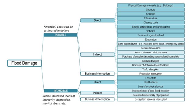
(Adapted from Flood Damage Assessment in Alberta, Best Practices and Guidelines, 2015)
Figure 8: Types of Flood Damage (not exhaustive).
Text version
Graphic listing a non exhaustive list of financial and social damages caused by a flood.
Flood damages may be assessed using a financial or economic impact approach. Financial impact refers to the sum of financial losses experienced by individuals or organizations as a result of a flood. The scale of the damage assessment should be defined by the flood-affected area. The outcomes of the assessment may be used to support flood management to reduce damages to properties and individuals. Beyond financial losses, at a larger scale, economic losses can be calculated as a sum of individual financial losses (and/or gains), to model economic losses for a region.
In many flooding situations, the actual damages incurred are less than the potential damages because sufficient warning is provided to the community such that mitigation measures can be taken in advance.
5.1. Tangible Direct Damage
There are several approaches to estimating tangible damage to buildings due to flooding.
Applying stage-damage curves is the most common and internationally accepted method for estimating tangible direct damage at urban scales. These stage-damage curves represent the relationship between flood depth and the estimate of absolute economic loss (in terms of currency) or relative loss (percentage of the estimated replacement value of property) of a building’s structure and contents. They may be derived by empirical (rely on data from past flood event) or synthetic techniques (conceptual approach and expert knowledge).
Probabilistic stage-damage functions are derived from stage-damage curves. They are commonly used to evaluate damages resulting from other natural hazards, e.g.: dam breaks, earthquakes, tsunami and fire. Probabilistic curves express the variability in the damage estimation process. These curves indicate the probability of damage exceeding certain spending thresholds (or damage states) based on various flood levels (McGrath et al., 2019).
Another method is through damage-frequency relationships. Damage-frequency relationships can be developed through direct examination of damage within the floodplain following flood events. If numerous estimates are available for a variety of flood events, a damage-frequency relationship could be developed from the data by plotting damage with respect to flood frequency or return period. However, the validity of using such relationships deteriorates with changes in land use over time as historical damage estimates based on historic land uses may not reflect the current-day land use or construction and contents costs.
Alternatively, a synthetic damage-frequency curve, from which average annual damages can be estimated for a given study area, can be used to assess damage. A synthetic damage-frequency curve can be produced from damage-frequency relationships by hydrologically determining various flood elevations for specific flood frequencies and synthetically deducing the damages that would result from these events. This method of computing a synthetic damage-frequency curve from damage-frequency relationships is considered to be the best approach for obtaining damage estimates based on current economic factors and has been proposed for use across Canada for riverine flooding.
While the above approaches are the most common, there are other methods of assessing other types of damages, for example using indicators or proxies.
5.1.1. Riverine Setting: Flood Damage Estimation Procedure
Buildings
Flood damages in areas prone to riverine flooding may be estimated using a four-part procedure composed of a hydrologic analysis, a hydraulic analysis, stage-damage calculations, and total damage calculations. This procedure is summarized in Figure 9.
Flows associated with various return period or probability events of interest are computed through the hydrologic analysis. Technical guidance on hydraulic and hydrologic procedures for preparing flood hazard maps can be found in the Federal Hydrologic and Hydraulic Procedures for Flood Hazard Delineation document.
The level of inundation for each property depends upon the grade of the property, the flood elevation and the floor heights above grade or a combination of these. The grade of the property may be established using a DEM derived from LiDAR, or alternatively, from ground level surveys or detailed topographic maps. The flood elevation may be derived from hydraulic flood modelling or from historical flood events (if available). Floor heights above grade can be established from building approval records, traditional field survey, or the use of street-level videos/photography.
Given an inventory of flood affected properties for a given return period event, and the depth of inundation at each property, stage-damage relationships can be applied to estimate the dollar value of direct content and structural damages. Indirect damages may also be estimated.
Total damage calculations involve computing the total damage for each return period flood event considering direct and indirect damages. Accordingly, total damage may be plotted as a function of return period or probability. Damage estimates may be expressed as expected value of annual damages. Annual damages are extrapolated from damage versus probability curves. Repeating the assessment with consideration of different mitigation measures will produce different expected values of annual damages. The reduction in estimated annual damages associated with each mitigation measure can be compared to the annualized project costs to support decision making and selection of flood mitigation options (Paragon Engineering Limited, 1984). Appendix 1 contains a breakdown of the aforementioned flood damage calculation procedures.
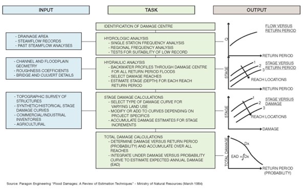
Figure 9: General Flood Damage Calculation Methodology
Text version
A figure describing the general flood damage calculation methodology
Damage to Other Infrastructure
In addition to buildings, there are a number of other assets that may potentially be exposed to flood damage. For example, direct and indirect damages may be inflicted upon:
- Roads and transport infrastructure;
- Parks and recreational facilities;
- Water, sewerage and drainage systems;
- Communication networks;
- Electrical power;
- Food/agriculture systems
Traditionally, most of these assets were publicly owned. However, the increasing trend towards privatization of services may have an influence on the costing methodology used to assess damages.
In general, the repair and replacement of roads and bridges represents the largest component of damages to public assets. The amount of damage caused depends upon the flood-related factors and the ability of the road to withstand flood conditions. Relevant factors include both the initial repair cost and the possibility of a significant reduction in the overall life of the road surface as a result of the flood.
Generally annual maintenance costs and other documented historical costs can be used to develop locally specific damage costs. Where this information is not available, data from other studies may need to be used. Depending upon the specific circumstances, these damages can vary greatly. Damages to assets categorized as “other infrastructure” generally range between 10% and 25% of direct damages to residential, commercial and industrial structures.
If damage estimates or actual damages can be determined for a specific return period and aerial extent of inundation, infrastructure damages can be interpolated for greater and lesser return periods based on the aerial extent of inundation (e.g.;., 75% or 125% of measured inundation area). Some judgement may be required in terms of land use mix and actual infrastructure components located within the flood hazard area.
5.2. Intangible and Indirect Damage
In addition to direct damage to property, a variety of secondary economic, social and environmental impacts are caused by flood events. The benefit-cost approach to disaster mitigation assessments theoretically requires a complete enumeration of all gains/benefits and losses/costs associated with a project (Ganderton, 2005). In practice, however, it is not possible to identify, quantify, and monetize all potential impacts.
The convergence of social, environmental, and economic issues with disaster mitigation under the umbrella of climate change adaptation has stimulated the field of risk assessment. Indirect and intangible impacts are receiving greater attention and, in some cases, are shown to be as substantial as direct costs (Joseph et al., 2014). Despite this, there remains very limited useful data upon which to assess indirect or intangible damages and no consensus on methodologies (Gall & Kreft, 2013). This leaves a tremendous gap between current theory and practice as well as great disparity within practice (a note of concern).
A major reason there are no practical examples of studies that reflect robust and detailed disaster loss estimate theory may be that it requires location-specific details that are not readily transferable. Thus the great time and cost make it prohibitive and the necessary data may be unattainable.
Due to these limitations, it is not feasible to arrive at the “total cost” of a flood by summing estimates for all the components. However, there are some general methods available that allow for the consideration of monetized indirect and intangible impacts, as outlined in the following sections.
5.2.1. Intangible Damages
Intangible damages are those for which establishing market value is extremely difficult. Human health impacts and damage to the environment both have intangible aspects. It is challenging to quantify intangible impacts caused by flood events. Floods do not lend themselves well to controlled studies that connect population and flood characteristics to outcomes (Tapsell, 2009). The intangible impacts of flooding on health and quality of life are highly dependent upon variables beyond the flood characteristics including an individual’s prior health, income, family and community support, preparedness and experience, and a host of other social indicators and behaviours. A 2017 report by IBI Group prepared for the City of Calgary describes a case study in which intangible damages were assessed.
Public Health and Quality of Life
There is little evidence to characterize most intangible outcomes of specific flood events/contexts (IBI Group, 2017). The process of quantifying the individual impacts relies on a large number of assumptions for each component variable. Monetization of these impacts requires further assumptions and transfer of values from other sources, most with no relation to flooding or the local context.
The available monetary values for all the impacts originate from various studies and contexts but ultimately they are all assumptions based on willingness-to-pay surveys (WTP) or choices and preferences of people somewhere. Complex calculations based on these values, estimated probabilities, and flood and population characteristics can lead to a value for each impact. However, this can obfuscate the origin of the data and the assumptions it contains. The end result will have questionable meaning or relation to stakeholders.
Furthermore, individually monetized impacts can yield values that are generally insignificant relative to the direct damages. Complex attempts to quantify injuries, disease, infection, and exposure can also lead to low values. This is not to suggest that these factors are not important, but the economic risks in this case are actually rather low. However, the impact on affected households is obviously considerable.
Two WTP studies related to flooding, and their applicability to Canada, are summarized in Appendix 5. At this time, an average value of $1,000 CAD per household per year is recommended. This amount can be adjusted based on the community profiles according to a risk scale of low ($700), average ($1,000), and high ($1,300). Further research is required to establish a Canadian WTP value.
Environment
Lasting environmental effects owing to water contamination from flooding will depend greatly on the characteristics of floodplain development. Restoration work conducted in or near waterbodies covered by the Fisheries Act necessitates offsetting costs to compensate for damaged habitat. It can be assumed that the costs of fish habitat offsetting measures are representative of the monetized damage corresponding to river bank stabilization projects. The total values from past events can be correlated to flow rates for those events and applied to the new flood data for each return period.
5.2.2. Indirect Damages
Indirect damages include costs of evacuation, employment losses, administrative costs, net loss of normal profit and earning to capital, management and labour, and general inconvenience. Indirect damages are best evaluated by developing a checklist of potential effects and methodically assessing each one. For example, the checklist would include the amount of use and the duration of interruption of transportation and communication facilities, the number of workers and farmers depending on closed plants, and the amount of business lost during a flood emergency. The magnitude of each effect may be estimated by interviewing those affected during recent floods, and unit economic values may be assigned by market analysis. Finally, the results may be summed to render a total value for indirect damages.
The complexity of the above evaluation process has led agencies to estimate indirect damages from direct damages based on percentages of direct damages. The ratios are chosen based on a review of the literature, empirical evidence, and expert opinion. For indirect damages that are associated with buildings, such as business disruption and residential displacement, another approach is to develop synthetic stage-damage curves.
Loss as a Percentage of Direct Damages
Indirect damages can range from 10% to 45% of direct damages for specific land use categories but are commonly calculated as 20% of direct damages. The Canada-Saskatchewan Flood Damage Reduction Program estimated indirect damages as 20% of all direct damages. This figure is in accordance with guidelines developed by the U.S. Soil Conservation Service who, in the past, suggested the following ranges for indirect damages:
- Agricultural: 5% to 10%
- Residential: 10% to 15%
- Commercial/Industrial: 15% to 20%
- Highways, Bridges, Railroads: 15% to 25%
- Utilities: 15% to 20%
Business Disruption Damage Curves
The impacts of major flood events on business are complex and varied. The main indirect damages suffered by businesses relate to disruption of business activities during the flood and restoration process or failure to re-open post event. This may occur as a result of damages to the business’ structure, equipment, and inventory; or because of access restrictions owing to evacuations, road closures, or loss of utility services. Methods for estimating the tangible indirect damages associated with business disruption are presented in Appendix 6.
There are a number of other factors that may influence indirect business damages including, for example, the cost of loans versus relief funds, the relationship between the business and the specific location, and the relationship between the business and other services and suppliers.
Residential Displacement Damage Curves
Structural damage from floodwaters, loss of critical services, or access restrictions owing to evacuation and road closures can all lead to residential displacement. During and after a flood event, affected residents will have to find alternative accommodations and incur extra personal expenses. Expenses may include restaurant meals, daily essentials, hotel costs, and extra fuel. Residents of buildings that require substantial repairs will require alternative accommodation for a longer period and incur costs for moving and rent.
Residential displacement costs are not often explicitly estimated in flood damage assessments but the required assumptions are relatively straightforward. Methods for estimating the tangible indirect damages associated with residential displacement are presented in Appendix 6.
Traffic Disruption
Floods can cause major traffic disruptions as a result of water on roadways, road closures, and required evacuation. Traffic delays also have associated financial and social costs. While traffic disruption is occasionally mentioned in literature related to flood impacts, it is rarely included in flood damage assessments. There are some studies on the economic impact of particular highway closures caused by flooding or landslides, but very few on urban flooding. Overall, detailed modelling of flood impacts on traffic is normally beyond the scope of flood damage estimation and is generally not warranted because the expected value is small in relation to other damages. Nonetheless, a description of the costs associated with traffic delays is included in Appendix 7 as well as a set of assumptions which may be employed to estimate vehicle disruption from municipal traffic modelling data.
Waste Disposal
The majority of flood-damaged property is disposed of in landfills. During a large-scale emergency clean-up operation, proper sorting of recyclable material or hazardous waste is often not performed. Additionally, current practice is to dispose of many items that might have been repaired in the past. This amounts to a great deal of waste from each flooded building.
Waste disposal has costs associated with collection, operation of the facilities, land usage, and environmental impacts.
The amount of post-flood waste created is assumed to be related to the total direct damages to buildings and contents. Damage calculations for waste removal can be calculated using past flood data. For example, City of Calgary landfills normally charge $113 per tonne for basic waste and $170 per tonne of construction and demolition materials when part of a mixed load (Calgary 2019). The amount for mixed load materials waste is assumed to represent the landfill cost for the flood-related waste. An additional $50 per tonne can be added to account for the time of private operators to bring the waste to the landfills. In general, damages associated with waste disposal equate to approximately 1.7% of estimated direct building and content damages.
Flood Fighting and Emergency Response and Recovery
Flood fighting and emergency response requires considerable effort by local administration and volunteers and it is often unaccounted for in damage estimates, or alternatively, included under indirect damages computed as a percentage of direct damage. The best source for costs related to this category is municipal records on past events. With a known amount for a given flood return period, or for an observed flood event, estimates for other return periods can be extrapolated using the inundation maps. The relationship between cost and direct damage or inundated developed area can be used.
6.0 Tools for estimating damage
In Europe and across North America, numerous computerized flood database and damage estimation models are employed for estimating flood damages. The majority of European models, with the exception of the UK are area-based models that calculate damage based on aggregated land use characteristics. In North America, the models are primarily object-based, calculating damages to individual buildings and include a large number of object types and corresponding flood damage characteristics to determine damages. Advantages of the object-based models is that they can control for varying building density and type, can be easily setup for rapid calculation over larger areas, and they enable scenario analysis. Smaller-scale studies in which the damage estimates of individual properties strongly affect the outcome will benefit from an object-based approach.
6.1. Large-Scale Analysis
There are several models in use across the country for flood damage estimation in Canada. The first computerized flood damage assessment system used in Canada was developed in the 1980’s. A number of software tools and their abilities are summarized in Appendix 8; much of the summary is based on research conducted by Lyle & Hund (2017).
All of these approaches have relied on stage-damage curves for damage estimation. Canadian studies have typically employed methodology aligned with Acres (1968), whereas U.S. studies have typically employed methodology aligned with the Flood Insurance Administration (FIA) (Federal Emergency Management Agency, 2016b). The differences between these approaches are highlighted in Table 3.
Given that major modifications to Hazus-MH would be required for effective and accurate use in Canada, it is recommended that the CanFlood, Alberta Provincial Flood Damage Assessment Tool (PFDAT) and Ontario Flood Damage (FLDDAM) programs be adopted for Canadian flood damage assessment studies.
| Acres approach | FIA Approach |
|---|---|
| Canadian data and experience. | U.S. regionalized experience (no Canadian verification). |
| Units by construction type relative to architectural/economic categories. | Units by construction type. |
| Contents damage evaluated through survey. | Contents damage expressed as a percentage of appraised value of structure. |
| Structural damage evaluated through detailed estimation of categories. | Structural damage expressed as a percentage of appraised value of structure. |
| Requires classification by category. | Requires individual appraisal of each unit. |
| Contents damage relates to general income grouping through unit categorization. | Contents damage is not related to income. |
| Considers basement damage. | Does not adequately consider basement damage. |
| Detailed evaluation for non-residential damage curves. | Non-residential damage curves inadequately represented. |
When using these software, it is necessary to consider the source of the stage-damage curves applied in the damage estimation. Stage-damage curves typically represent an ‘average’ structure of a given category. Thus, when considering a single structure, the damage estimate contains uncertainty, based on the aggregation of the results from structures of a similar type, but different valuations and sizes. This uncertainty increases with increasing water depth. For example, variability of Ontario stage-damage curves from a sample of 76 one-storey residences with basements found a variability of ~$10,000 at a water depth of 0 m and ~$25,000 at a flood depth of 2.4 m (Paragon Engineering Limited et al. 1985; McGrath et al., 2019). For larger-scale analyses (e.g.: community level), the local inaccuracies can be expected to average out to a certain extent. In addition, many communities do not have sufficient resources to develop their own curves and may adapt those developed in other communities or regions. This can also lead to uncertainty in the resulting damage estimate. Thus, further refinement of the programs is recommended in order to incorporate the desired functions and ease-of-use for use in future Canadian studies.
A lack of detailed building inventory can lead to challenges in building or community level damage estimation and risk assessment. The challenges are largely related to the quality of data available and the amount of data processing required. In most municipalities these challenges can be easily overcome. However, in larger urban centers containing areas of dense and multi-use building arrangements, difficulties can arise.
6.2. Individual Building Analysis
The tools described in the previous section are also capable of object based, or individual building level analysis in addition to the large-scale analysis, however, individual building results must be used with caution, especially if stage-damage curves from other regions have been employed.
Xactimate® is a software tool used for individual building damage estimation as well as municipal level evaluations and claims handling. This software is used by many Canadian (and U.S.) insurance companies as well as restoration contractors and adjusters. The Xactimate system allows for digital data entry of a buildings’ dimensions, rooms and contents and is able to access an extensive database of costing tables and price lists. In addition, users can upload regional labour rates and price lists.
6.3. Database Issues and Considerations
Good database design is essential for damage estimation. The design should consider the necessary attributes required and limit user response options through inclusion of drop-down menus to promote standardization.
One major issue in the damage estimation process relates to the fact that assessed value within records includes land and improvements and therefore one cannot apply standard Content to Structural Value Ratios (CSVR) as it will overstate the content value. For multi-tenant buildings there is no way of disaggregating assessed value by specific unit or use such that one can apply an appropriate CSVR (Hence, the Hazus-MH and HEC-FDA damage estimation methodologies cannot be applied). Business type descriptors for retail are typically not subdivided into specific types (i.e., shoes, clothing, electronics, paper products, groceries), and therefore do not allow for the fine-grained contents assessment by specific business type.
Common data quality issues and possible solutions, as well as a discussion of available internet tools to assist in building classification can be found in Appendix 9. Future development of a comprehensive flood damage database would benefit from gathering of the following information (e.g. through tax assessments).
7.0 Stage-damage curves
Damage to residential and commercial properties and contents caused by inundation during flood events can be assessed using stage-damage curves. Direct flood damages should be estimated separately for residential and non-residential structures. Additionally, structural damages should be estimated separately from content damages.
Structural damage refers to damage to the building and to stationary building components such as furnaces, hot water heaters, carpeting, etc. Content damage refers to damage to moveable contents within a structure (McBean et al., 1986). Contents and structure data should be collected from a representative sample of units located within the defined flood hazard area. Effort should be expended to identify units that are “typical” of their residential classification in terms of size, assessed value, and apparent quality.
Baseline damage estimates should reflect total potential damages and should not consider any existing mitigation measures. Essentially, this approach assumes failure of existing mitigation structures and absence of any non-structural mitigation measures. This methodology permits benefit/cost analyses of proposed mitigation options against the baseline condition.
Sample data collection forms for residential (Appendix 10), and commercial properties (Appendix 11) are included.
Stage-damage curves, developed for the City of Calgary in the IBI Group and Golder Associates 2015 report, for residential and commercial properties are included in Appendix 12 and Appendix 13 respectively. The content item and price list utilized to develop the stage damage curves is found in Appendix 14.
7.1. Residential Stage-Damage Curves
Potential damages vary substantially based on type of use (building occupancy classification), construction materials, construction techniques and quality, and the quantity and nature of contents located within the structure. Therefore, it is necessary to formulate a classification scheme capable of encompassing considerable variations in housing types found throughout the study area. Accordingly, stage-damage curves may be developed for each category of the classification scheme. A number of residential classification schemes have been developed from previous Canadian studies and projects, a summary and example photographs are found in Appendix 15.
Exterior finishing materials show some variation by region: in the western provinces there are more stucco and siding materials, brick is used extensively throughout Ontario, while clapboard and siding are the predominant materials in Quebec and the Atlantic provinces. Exterior materials are generally not considered in flood damage estimates as they generally suffer little to no damage under general riverine flooding conditions. High velocity flows, ice and debris in the flood water can contribute to greater exterior damage.
7.1.1. Development of Content Damage Curves
In general, it is recommended that region-specific content damage curves are developed to reflect the characteristics of the study area. Additionally, content damage curves should be developed separately for each storey (basement and main level), and each residential structural category, calculated on a dollar-per-square-metre-of-floor-area ($/m2).
Following the development of the contents inventory, content stage-damage curves may be calculated for each storey and each class of residential dwelling unit. The calculated flood damages occurring at each depth of flooding above floor level should be averaged on a dollar- per-square-metre-of-floor-area basis.
In flood-affected areas where large high-value, single-family homes represent a small percentage of the total inventory (less than 1%), it is not possible to obtain a sufficiently large sample of content inventory. In these cases, the content damage curves may be estimated at a premium of 1.44 over the next highest class structures.
Garden tools, garden furniture, and garage contents should be inventoried as part of the residential contents survey (IBI Group & Golder Associates, 2015). To account for landscaping and yard clean-up costs, guidance is provided in Appendix 16 for different classes of properties. Appendix 16 also contains a description of studies in which external damages were considered in flood damage estimates.
7.1.2. Development of Structural Damage Curves
The structural characteristics of residential units in each class should be determined through field inspection by qualified architectural personnel and consultation with the local building industry. Typical basement unit floor areas and first floor areas may be determined for each class of residential unit from municipal assessment data, otherwise, interviewers should collect information on building floor areas, exterior finishes, building and room perimeters, and types of interior finishes (IBI Group & Golder Associates, 2016).
The average floor areas data collected through field inspection surveys can be combined to develop the profile of typical units in each residential classification.
Estimates of unit prices for cleaning, replacing and/or repairing flood damaged materials may be obtained from local suppliers and contractors. All structural damage curves should reflect the costs of cleaning, repair, and restoration estimated on the basis of current local material and labour costs. It should also include the cost of removing residual standing water, sediment, removal, disposal of damaged items, structural drying and sanitization, final inspection and testing for dryness and residual contamination.
It is common practice to remove and replace all non-structural materials that have been in contact with floodwater for residential flood remediation. In addition, due to moisture wicking upwards through semi-permeable building materials, very high ambient humidity levels inside structures, and the probability of mold growth on common residential finish materials, it is now a recommended and generally observed practice to remove virtually all finish materials on floor levels that experience any substantial duration and depth of flooding with Category 3 waterFootnote 1.
The major structural components of a typical dwelling unit, if properly maintained, have a life expectancy that virtually defies application of arbitrary depreciation rates. In general, deterioration is related primarily to wear of finishes, wall and floor coverings, and similar materials, as long as these materials in the typical home are generally well-maintained. Consequently, no depreciation estimates need be applied to replacement and/or restoration values used to construct the structural stage-damage curves.
Based on dwelling unit characteristics and unit prices, damage for each 300 mm of flooding should be estimated for each class of residential unit, floor level, and structural type.
Attached and detached garage damages should be included for all building classes excluding mobile homes, low-rise apartments, and high-rise apartments. Structural damages for low- and high-rise apartment parkades should be calculated separately on a structure-specific basis..
7.2. Non-Residential Stage-Damage Curves
Non-residential buildings including commercial/industrial and institutional establishments, include inventory, equipment, and building damage as well as clean-up costs. As with residential structures, content and structural damages should be calculated separately. Due to the range and diversity of activities associated with non-residential buildings, this group does not demonstrate the same uniformity as the residential grouping. Consequently, categorization is much more complicated and it is necessary for similar types of commercial activities to be grouped together.
Appendix 17 provides a detailed description of the commercial/industrial classes used in the Alberta Provincial Flood Damage Assessment study (IBI Group & Golder Associates, 2015). The corresponding commercial damage curves are presented in Appendix 13 and detailed descriptions of restoration activities and assumptions employed in constructing these curves and the representative commercial industrial establishments can be found in the 2015 report by IBI Group and Golder Associates.
7.2.1. Content Damage Curves
Commercial contents are primarily composed of inventory. Furthermore, commercial content damage estimations should be based on the non-salvageable portion of affected inventory.
In general, reported levels of salvageability are quite low reflecting the same restoration difficulties, health and safety concerns, and cost issues described for residential contents. Fixtures and furnishings damages should reflect replacement costs and commercial content inventories should reflect replacement (wholesale) values.
7.2.2. Structural Damage Curves
Structural damage curves for non-residential buildings were developed from first principles based on a six-fold classification scheme. The six categories in the classification scheme include office/retail, industrial/warehouse, hotel/motel, institutional, office towers, and multi-level parkades.
Structural damage curves can be constructed using actual building plans to determine areas and levels of finishes. Estimates of unit prices for replacing and/or repairing flood damaged materials may be obtained from local suppliers and contractors. Structural damage curves should reflect the costs of repair or restorations estimated on the basis of present-day regional material and labour costs.
One difference with respect to restoration of non-residential versus residential structures is the practice of “stepped” rehabilitation versus wholesale residential renovation at low levels of flooding. This is due to a number of factors including:
- The use of more durable materials that have a higher level of salvageability;
- Cleaning and structural drying is easier to implement;
- As commercial buildings are a for-profit venture, owners attempt to minimize repair costs and downtime; and
- Insurers exercise a higher degree of caution in residential remediation due to potential liability relative to health and occupancy issues.
Multi-Level Below-Grade Parkades
Stand-alone multi-level below-grade parkades, along with those associated with mid- and high- rise offices and residential buildings, constitute a new damage category not previously encountered in the literature. A value of $215/m2 is suggested to estimate damages for structures that belong to this category (IBI Group & Golder Associates, 2015) as further described in Appendix 18. Depending on the time of day, advance warning and neighborhood, the type and cost of vehicles that may be in the parkade will vary. This may need to be considered individually.
7.2.3. Industrial Damages
A field survey of specific industrial establishments is recommended employing the sample questionnaire contained in Appendix 11. With regard to the survey, one should (Ontario Ministry of Natural Resources, 2007):
- establish a contact for the plant manager or foreman;
- review with the contact, the nature and vertical placement of all major equipment and inventories;
- determine if inventories vary with season;
- determine the value of down-time in relation to revenue, to help assess indirect costs;
- assess structural damage that would be incurred; and
- if flood forecasting opportunities exist, determine what adjustments are enacted to decrease damage (another measure of indirect cost)
If the level of effort does not permit detailed damage surveys, it is suggested that the Province of Alberta 2015 Commercial/Industrial/Institutional Depth-Damage Relationships provided in Appendix 13 be employed with indexing to account for inflation and regional cost differences.
7.2.4. Agricultural Damages
Agricultural damages include damages to crops, soil, equipment and implements, farm supplies (such as fertilizer and seed), farm structures, and livestock mortality. They are primarily dependent on the timing and duration of flooding, in contrast to other damages, which primarily depend on the depth of flooding. Losses associated with damage to crops can be adjusted according to the type of crop and size of area inundated.
For each crop type in the study area, data requirements include:
- The yield and market value per hectare (acre) of land for each crop type;
- The flood-free gross income, calculated using adjusted normalized prices (if required) for each crop type (refer to Section 8.1 on price adjustments)
- The costs of production, broken down by month;
- The monthly probability of flooding for each flood depth, a value that can be estimated by a hydrologist;
- The monthly damage rates (also referred to as crop loss functions), a value up to 100% of the total production value of the crop obtained based on the history of flooding in agricultural areas for each month in which flooding occurs (these values can be derived from literature reviews and interviews with farmers and local agricultural specialists); and
- The aerial extent of each crop type in the study area.
Procedures for estimating damages to crops, livestock, and barns and outbuildings are presented in Appendix 19. The recommended coding for agricultural crops, livestock and buildings and equipment are shown in Appendix 15, Table F-8.
7.2.5. Unique Structures/Uses
Not all structural types or uses will fit into the standardized residential, commercial and industrial classifications established for stage-damage curves development. These structures include very specialized buildings like hospitals and sports facilities/arenas and uses such as campgrounds, parks and golf courses. In these instances, potential damages should be estimated from first principles employing data collection instruments to determine direct and indirect damages, similar to the methods employed for constructing the standardized contents and structural damage curves. Appendix 20 describes a case study in which this methodology was employed.
7.3. Limitations in Stage-Damage Curves
A brief discussion of the uncertainty associated with structural classification schemes and stage- damage curve development is presented in Appendix 21. Stage-damage curves are presented as a single relationship for a given water depth, a given dollar value of damage and typically exclude other damage-inducing parameters such as flow velocity, debris and contaminants.
7.3.1. Damage due to Velocity
When calculating damage in areas where velocity is a factor, depth should be calculated relative to the bottom of the floor beam of the lowest floor (the main level) in coastal and lake flooding, whereas the top of the finished flooring of the lowest floor is used as the reference level with riverine flooding (Federal Emergency Management Agency, 2006).
Specific calculations for structures under high-velocity flows must be conducted to determine whether structural failure will occur for given flooding characteristics (Paragon Engineering Limited, 1985). FEMA functions showing building collapse potential as a function of wave induced velocity and depth are shown in Appendix 3.
To estimate damage as a result of total destruction, the total structural and content damages that would result from inundation alone should be estimated for the basement and first floor and multiplied by a value of 2.86. Alternatively, the replacement cost of the structure may be estimated using the assessed value of the property under normal market conditions (less the value of the land) and added to the total insured value of the contents of the structure. These estimates may be converted to a per-square-metre basis to facilitate further analyses and the development of standardized damage functions.
If it is determined that a structure is not expected to collapse, then damages can be estimated based on inundation alone.
In the event of a mobile home collapse, or other type of home without a basement, it is assumed that none of the building contents would be saved or moved to higher ground. Therefore, damages may be estimated using the methods described in Section 7.1. Note that mobile homes need not be adjusted for the value of the lot since they are commonly leased.
8.0 Future adjustments and regional indexing
8.1. Updating to Current Year Dollars
Stage-damage curves should continually be updated to represent current-year dollars and take inflation into account. As a result of inflation, past damage-curve estimates may not be directly applicable to future flood events. However, since changes in a variety of prices are regularly tracked by Statistics Canada, it is possible to develop an appropriate index to update base-year estimates to accommodate relevant price changes over time.
Damage estimates from any previous base year can be updated to a new base year. To do so, one simply multiplies the damage values by the ratio of the current index value over the index value from the previous base year, as followsFootnote 2:
Current Damages = Base Year Damages x (Current Year Index / Base Year Index)
8.1.1. Available Measures of Price and Spending Change
Different procedures are required for the adjustment of residential versus non-residential damages, and similarly for the adjustment of contents versus structural damage. Accordingly, a number of price and spending change measures must be employed to adjust damage estimates to reflect current-year dollar values. These measures include the consumer price index (CPI), construction price indexes, and the survey of household spending (SHS). Descriptions of each price and spending measure are included in Appendix 22.
8.1.2. Updating Residential Content Damages
The “all-items” CPI is an aggregated index reflecting price movements of a collection of products and services purchased by consumers. The “all-items” CPI is commonly used to update content damage estimates from a previous year. However, the use of this index introduces error into the flood damage analysis since flooding affects only a particular group of items from the CPI basket.
To account for the aforementioned shortcoming of the “all-items” CPI, the adjustment computations can be conducted by selecting only the sub-categories of the “all-items” CPI directly related to flood damage; individual CPI values are available for all sub-categories of the “all-items” CPI. This procedure is described in Appendix 23, although it is not the preferred approach for updating residential content damages.
It is important to note that the CPI is intended to represent pure price changes of standardized goods. It intentionally does not account for changes in quality or technology. Computers and other electronics illustrate this effect; the index price of a computer with an unchanging processing capability will drop substantially over a relatively short time. However, because the technology continues to improve, the average new purchase price may be unchanged or possibly increase. Additionally, the individual CPI indexes cannot account for changes in consumer behaviour caused by changing prices or incomes.
For example, if clothing prices drop or income increases, a household may buy more clothing but have a clothing inventory with a value that did not decrease.
A better measure of the change in household content value over time is the Statistics Canada SHS. Average household expenditures are measured annually in categories similar to the CPI and are available at the provincial level. For example, if average household spending on televisions remains the same over a period of ten years, it is assumed that this dollar amount represents the value of television equipment in a household, even if the CPI of an unchanging television set fell substantially.
The results of the SHS can be used to index the residential content value between two years in the same way as the CPI by using the weighted value of spending for the flood-affected categories. The procedure is demonstrated in Appendix 23.
8.1.3. Updating Non-Residential Content Damages
The contents of commercial, industrial, and institutional buildings susceptible to flood damage are not reflected by the CPI basket in either composition or weighting. Furthermore, spending surveys do not exist for non-residential categories and the assumed relationship between household spending and content value does not apply to commercial structures.
Without conducting new content surveys for each commercial structure category, a general index that avoids product-specific omission of quality changes is required. As part of the CPI, Statistics Canada provides the special aggregate “Goods” to exclude services, shelter, and energy that would not be affected by flooding. As the components of this aggregate are weighted by province according to the SHS, it can be assumed to represent the general composition of commercial contents, including non-durables that are insignificant in value at any one time in a household but may represent a significant value of commercial inventory.
Therefore, the following formula may be employed to update commercial content damages:
Current $ = Base Year $ X (Current CPI Goods Aggregate / Base CPI Goods Aggregate)
8.1.4. Updating Structural Damages
Structural flood damage is the estimated cost for repair and/or replacement of building components damaged by flooding. The price of construction/restoration is dependent on the building type. The main building type categories are:
- House (single dwellings, semi-detached, and row-houses);
- Apartment (vertical attached dwellings); and
- Non-Residential (commercial, industrial, and institutional).
Statistics Canada regularly publishes construction price indexes for the above building type categories, as well as infrastructure construction. Restoration of a flood-damaged building is not equivalent to new building construction. For example, structural items such as wall studs, foundation concrete, and electrical wires may not be replaced after a flood. However, the construction price indexes are the most relevant measure of changes in real market price for construction work. These indexes cover all representative construction materials, general and trade contractors’ labour, equipment, overhead, and profit while excluding the cost of land, design, development and real estate fees.
Base year structural damage estimates can be updated using the most recently published construction price index for the corresponding building type.
8.1.5. Updating Damages Summary
A summary table of recommended methods for updating damage estimation curves developed in this report is provided in Table 4.
| Damage Type | Index Used | Index Components and Weighting | New Damages Formula X=Base Year Damages, wi = Weight |
|---|---|---|---|
| Contents: Residential | Survey of Household Spending | Household Furnishings & Equipment 59% Clothing & Accessories 21% Recreation 20% |
|
| Contents: Non-Residential | Consumer Price Index | Goods Special Aggregate | |
| Structure: Residential – House | New Housing Price Index | N/A | |
| Structure: Residential – Apartment | Apartment Building Construction Price Index | N/A | |
| Structure: Non-Residential | Non-Residential Building Construction Price Index | N/A |
8.2. Regional Adjustments
In addition to changes in price over time, there are often substantial regional price differences across markets that should be recognized. Demographic, economic, and geographic factors all influence the price of goods and services at the regional level. Unlike the temporal data from Statistics Canada, regional price data is not regularly published from a single source.
8.2.1. Adjusting Content Damages
The replacement price of flood-damaged contents may vary between communities and regions. The CPI measures the changes in price of an equal basket of goods in the same place at different times. Measuring the price of that equal basket in different places at the same time allows for regional price comparisons. A spatial price survey can be used to create an index to compare the costs of goods between communities. With this type of spatial survey, item categories can be selected and weighted to reflect the results of the contents survey that the damage curves are based on.
In the absence of comprehensive spatial price surveys, there are several other sources of price differences. For a limited number of locations across the country, Statistics Canada publishes inter-city indexes of price differentials of consumer goods and services (Statistics Canada, 2017). With category weighting applied, this index could be used to adjust damage amounts between listed cities. Other cost of living surveys may be available with sufficient detail to provide a basis for creating a flood-damaged contents index.
It should be noted that the use of a spatial price survey assumes that there are similar household contents within each class of housing between the locations being compared, but that replacement cost may be different. If applying a content damage curve from another region, there may be discrepancies in the composition of household goods. As with temporal adjustments, the SHS can be used to estimate differences in the value of household contents between provinces if pronounced differences are expected.
8.2.2. Adjusting Structural Damages
The cost of labour and materials required for restoration of buildings after a flood will vary with local market conditions and capacity. Annually published construction cost guides provide a basis for indexing structural damages between communities. An appropriate cost guide would exclude land price and soft costs not relevant to flood restoration. A good example is Altus Group’s Canadian Cost Guide. The guide provides average construction prices for a location in six regions as well as an index for other locations within that region. Costs are provided for six building types with multiple subcategories and quality levels, allowing for the use of an index for each type of structural damage curve. One can simply divide the average cost in the study area by the cost from the location the curve was developed to determine the appropriate multiplier.
9.0 Case studies
The following links represent flood damage assessment studies for various-sized centres:
Alberta Environment and Parks: Provincial Flood Damage Assessment Study: Town of Canmore: Damage Estimates
Alberta Environment and Parks: Provincial Flood Damage Assessment Study: Town of Okotoks: Damage Estimates
Alberta Environment and Parks: Provincial Flood Damage Assessment Study: Town of Whitecourt: Damage Estimates
City of Calgary: Flood Mitigation Options Assessment – Phase 1 & 2
City of Vancouver Coastal Flood Risk Assessment Phase II Final Report. 2015 (PDF 7.90 MB), Lyle, Tamsin, Graham Long, and Christian Beaudrie
Evaluating Quantitative Flood Risk Assessment Tool in Manitoba and its Application to Policy (PDF 3.70 MB). Suzanne Houlind.
Integrated Flood Hazard Management - River Flood Risk Mitigation Options - Final Report (PDF 74.2 MB).”2017 KWL.
Lower Mainland Flood Management Strategy Project 2: Regional Assessment of Flood Vulnerability (PDF 53.4 MB) - Final Report.” NHC. 2016
Provincial flood damage assessment study City of Calgary: assessment of flood damages
10.0 References
Acres Limited. (1968). Guidelines for Analysis, Volume II Flood Damages. Niagara Falls ON: Government of Canada and Ontario Joint Task Force on Water Conservation Projects in Southern Ontario.
Bonsal, B.R., Peters, D.L., Seglenieks, F., Rivera, A., and Berg, A. (2019): Changes in freshwater availability across Canada; Chapter 6 in Canada’s Changing Climate Report, (ed.) E. Bush and D.S. Lemmen; Government of Canada, Ottawa, Ontario, p. 261–342.
Brémond, P., Grelot, F., & Agenais, A.-L. (2013). Review Article: Economic evaluation of flood damage to agriculture – review and analysis of existing methods. Natural Hazards and Earth System Science, 13 (10), 2493–2512.
Bubeck, P., & Kreibich, H. (2011). Natural Hazards: direct costs and losses due to the disruption of production processes. Potsdam: GFZ, Helmholtz Centre Potsdam.
Burrell, B.C, Huokuna, M, Beltaos, S. (2015) Flood Hazard and Risk Delineation of Ice-Related Floods: Present Status and Outlook, Conference: 18th Workshop on the Hydraulics of Ice Covered Rivers, Quebec City, QC
Calgary 2019. Landfill Rates. Retrieved from: Landfill materials and rates, accessed 10/28/2019
Dachis, B. (2015). Tackling traffic: The economic cost of congestion in metro Vancouver. C.D. Howe Institute eBrief 206.
Defra/Environment Agency, & Flood and Coastal Defence R&D Programme. (2004). The Appraisal of Human related Intangible Impacts of Flooding (No. FD2005/TR). Defra.
Environment and Climate Change Canada. (2017). Hurricane Hazel.
Erickson, T. B., Brooks, J., Nilles, E. J., Pham, P. N., & Vinck, P. (2019). Environmental health effects attributed to toxic and infectious agents following hurricanes, cyclones, flash floods and major hydrometeorological events. Journal of Toxicology and Environmental Health, Part B, 22(5-6), 157-171.
Federal Emergency Management Agency. (2005) Effects of Long and Short Duration Flooding on Building Materials.
Federal Emergency Management Agency. (2006). Hazus - MH Technical Manual. Washington DC: FEMA.
Federal Emergency Management Agency. (2016a). National Flood Insurance Program.
Federal Emergency Management Agency. (2016b). National Flood Insurance Program: Flood Hazard Mapping.
Gall, M., & Kreft, S. (2013). Measuring What Matters? A Suitability Analysis of Loss and Damage Databases for the Climate Change Convention Process.
Ganderton, P. T. (2005). “Benefit–Cost Analysis” Of Disaster Mitigation: Application As a Policy And Decision-Making Tool. Mitigation and Adaptation Strategies for Global Change, 10(3), 445–465.
Government of Alberta (2019) Flood Hazard Mapping, retrieved 10/01/2019
Government of New Brunswick. (2017). Coastal Flooding and Storm Surges.
Greenan, B.J.W., James, T.S., Loder, J.W., Pepin, P., Azetsu-Scott, K., Ianson, D., Hamme, R.C., Gilbert, D., Tremblay, J-E., Wang, X.L. and Perrie, W. (2018): Changes in oceans surrounding Canada; Chapter 7 in (eds.) Bush and Lemmen, Canada’s Changing Climate Report; Government of Canada, Ottawa, Ontario, p. 343–423.
Hansen, W. J. (1987). National Economic Development Procedures Manual-Agricultural Flood Damage (No. IWR-87-R-10). Fort Belvoir VA: Army Engineer Institute for Water Resources Fort Belvoir.
HDR Inc. (2015). Current and Projected Costs of Congestion in Metro Vancouver, Final Report. Translink.
IBI Group Professional Service (2017). The Flood Mitigation Options Assessment, prepared for The City of Calgary.
IBI Group, & ECOS Engineering Services Ltd. (1982). Phase II-B Flood Damage Estimates, Fort McMurray Flood Damage Reduction Program. Fort McMurray, AB: Alberta Environment and the City of Fort McMurray.
IBI Group, & Golder Associates. (2015). Provincial Flood Damage Assessment Study. Calgary AB: Government of Alberta, Environment and Sustainable Resource Development.
IBI Group, & Golder Associates. (2016). City of Calgary Flood Mitigation Options Assessment. Calgary AB: City of Calgary, Water Resources Division.
iTRANS Consulting Inc. (2006). Costs of Non-Recurrent Congestion in Canada Final Report, Transport Canada Economic Analysis (No. TP 14664E). Ottawa ON: iTRANS Consulting Inc.
James, T.S., Henton, J.A., Leonard, L.J., Darlington, A., Forbes, D.L., and Craymer, M. (2014). Relative Sea-level Projections in Canada and the Adjacent Mainland United States; Geological Survey of Canada Open File 7737, 72p. doi: 10.4095/295574
James, T.S., Henton, J.A., Leonard, L.J., Darlington, A., Forbes, D.L., and Craymer, M. (2015). Tabulated Values of Relative Sea-level Projections in Canada and the Adjacent Mainland United States; Geological Survey of Canada Open File 7942, 81p.
Joseph, R., Proverbs, D. G., Lamond, J. E., & Wassell, P. (2014). The Costs of Flooding on Households. In Water Resources in the Built Environment: Management Issues and Solutions (pp. 249–257).
Joseph, R., Proverbs, D., & Lamond, J. (2015). Assessing the value of intangible benefits of property level flood risk adaptation (PLFRA) measures. Natural Hazards, 79(2), 1275– 1297.
Lemmen, D. S., Warren, F. J., James, T. S., Clarke, C. S. L. M., Canada, & Natural Resources Canada. (2016). Canada’s marine coasts in a changing climate.
Leonard, L. J., Rogers, G. C., & Mazzotti, S. (2012). A preliminary tsunami hazard assessment of the Canadian Coastline (No. 7201).
Lyle, T. S., & Hund, S. V. (2017). Way forward for risk assessment tools in Canada (No. 8255). Geological Survey of Canada.
McBean, E., Fortin, M., & Gorrie, J. (1986). A critical analysis of residential flood damage estimation curves. Canadian Journal of Civil Engineering, 13(1), 86–94.
McGrath H, El Ezz AA, Nastev M. Probabilistic depth–damage curves for assessment of flood-induced building losses. Natural Hazards. 2019:1-4.
Mekis, É., Vincent, L. A., Shephard, M. W., & Zhang, X. (2015). Observed trends in severe weather conditions based on humidex, wind chill, and heavy rainfall events in Canada for 1953–2012. Atmosphere-Ocean, 53(4), 383-397.
Messner, F., Penning-Rowsell, E., Green, C., Meyer, V., Tunstall, S., & van der Veen, A. (2007). Evaluating flood damages: guidance and recommendations on principles and methods (No. T09-6–1). Helmholz Unweltforschungszentrum (UFZ).
NOAA. (2016). Ocean Facts.
NOAA. (2017a). National Tsunami Warning Centre and Pacific Tsunami Warning Centre.
NOAA. (2017b). National Weather Service.
Ontario Ministry of Natural Resources. (1997). Natural Hazards Training Manual: Provincial Policy Statement: Public Health and Safety Policies 3.1. Ontario Ministry of Natural Resources.
Ontario Ministry of Natural Resources. (2007). Flood Damage Estimation Guide, 2007 Update and Software Guide. Toronto ON: Ontario Ministry of Natural Resources.
Paragon Engineering Limited. (1984). Flood Damages: A Review of Estimation Techniques. Ottawa ON: Ontario Ministry of Natural Resources.
Paragon Engineering Limited. (1985). Development of Flood Depth-Damage Curves for Residential Homes in Ontario. Ottawa ON: Environment Canada, Ontario Ministry of Natural Resources.
Penning-Rowsell, E.C, Johnson, C, Tunstall, S, Tapsell, S, Morris J, Chatterton, J, Coker A, Green C (2003), The Benefits of flood and coastal defence: techniques and data for 2003, Flood Hazard Research Centre, Middlesex University
Saskatchewan Forage Council. (2017). Forage Market Price Discovery - Saskatchewan. Scawthorn, C., Flores, P., Blais, N., Seligson, H., Tate, E., Chang, S. Lawrence, M. (2006).
Shephard, M.W., Mekis, E., Morris, R.J., Feng, Y., Zhang, X., Kilcup, K. and Fleetwood, R. (2014):Trends in Canadian short-duration extreme rainfall: including an intensity-duration-frequency perspective; Atmosphere-Ocean, v. 52, p. 398–417
Statistics Canada. (1996). Catalogue no. 62-557-XPB Your Guide to the Consumer Price Index (PDF, 400 kb),. Statistics Canada. (2016). Weighting Diagram of the Consumer Price Index - 2011 Basket at January 2013 Prices, Canada, Provinces, Whitehorse and Yellowknife. Retrieved February 8,2018.
Statistics Canada. (2017). Inter-city indexes of price differentials of consumer goods and services, Table 326-0015. Retrieved February 8, 2018.
Shephard, M. W., Mekis, E., Morris, R .J., Feng, Y., Zhang, X., Kilcup, K., & Fleetwood, R. (2014). Trends in Canadian short-duration extreme rainfall: Including an intensity–duration–frequency perspective. AtmosphereOcean, 52(5). doi:10.1080/07055900.2014.969677
Steward, R.M. (2007). Community Perspectives of Flood Risk and Social Vulnerability Reduction: The Case of the Red River Basin (PDF 6.80 MB). University of Manitoba (PhD Thesis).
Tapsell, S. (2009). Developing a conceptual model of flood impacts upon human health (No. T10- 9–2). Middlesex University.
United States Department of Agriculture Soil Conservation Service. (1972). TSC Technical Note– Watersheds – UD-28. USDA.
Vincent, L. A., Zhang, X., Mekis, É., Wan, H., & Bush, E. J. (2018). Changes in Canada's climate: Trends in indices based on daily temperature and precipitation data. Atmosphere-Ocean, 56(5), 332-349.
Zhang, X., Flato, G., Kirchmeier-Young, M.,Vincent, L., Wan, H., Wang, X., Rong, R., Fyfe, J., Li, G., Kharin, V.V. (2019):Changes in Temperature and Precipitation Across Canada; Chapter 4 in Bush, E. and Lemmen, D.S. (Eds.) Canada’s Changing Climate Report. Government of Canada, Ottawa, Ontario, pp 112-193.
Appendix 1 – Breakdown of Flood Damage Calculation Steps
-
Step 1 – Flood Hazard Mapping
Develop flood hazard maps, for multiple return periods. Refer to the Federal Hydrologic and Hydraulic Procedures for Flood Hazard Delineation for details. The output of the flood hazard map provides information on the flood extent, depth, and velocity for each pixel on the map based on the modelled scenario(s).

-
Step 2 – Identify Affected Properties
Working with local community assemble inventory of features that could be impacted, including buildings, infrastructure, population.
For the buildings, identify attributes of the building, including occupancy type, age, height of first floor, number of stories, presence/absence of basement, etc. Identify those buildings that are within the floodway, flood fringe, and adjacent-to-areas. Basement damages could occur even if the property is outside of the flood hazard area because of sewer backup or ground seepage. Consequently, properties in the adjacent-to-areas should be included for damage estimates.
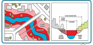
-
Step 3 – Compute Direct Damage
Identify existing local stage-damage functions for each building class identified in Step 2. Develop local functions. If resources are not available, identify similar functions and compute regional adjustments. Establish a mechanism to check and review selected/ developed stage-damage functions. Compute damage estimates for all identified properties and repeat for each return period. A cumulative total for each return flood event is computed. The total potential direct damage resulting from a 1:100 year flood, 1:50 year flood, etc. is established. Plot total damage as a function of return period or probability. Estimated Annual Damages (EAD) are extrapolated from damage versus probability.
Components to compute damage:
* Damage Curve Height = Flood Elevation – (Main Floor Height Above Grade + Grade Elevation)
* Main Floor Damage = Dollar Value On Curve Equal To The Damage Curve Height* Total Damage = Basement Damage + Main Floor Damage
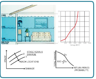
-
Step 4 - Evaluate Indirect Damage
Once an assessment of the potential damages to the affected properties has been made, the indirect damage can be estimated. It is common practice that the indirect damages for residential and commercial property be estimated as a percentage of the direct damage. Values generally range from 20% to 40% depending upon the specific circumstances.
In addition a percentage is also attributed to infrastructure, highways and utilities unless these damages can be estimated from first principles by the municipality. It should be noted that the indirect percentages should be re-assessed for each of the flood affected communities and they should be based on the local situation assessment. Indirect damages should be reassessed over time especially if new mitigation measures are proposed
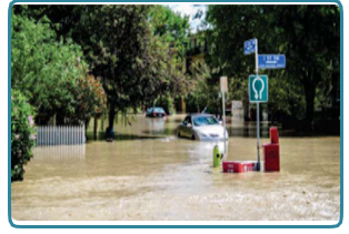
-
Step 5 – Compute Total Damages
The total damage cost for each return flood is the sum of all direct and indirect damages.
Total damages = direct damages + indirect damages

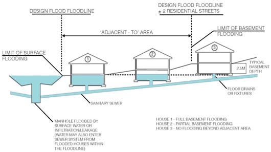
Figure A-1: Adjacent-to Area Figure (IBI Group)
Text version
A figure describing the breakdown of flood damage calculation steps.
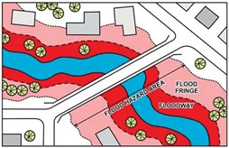
Figure A-2: Flood Hazard Area (source: Government of Alberta, 2019)
Text version
Figure showing the cross-section of a flood hazard area.
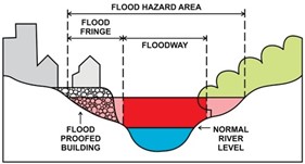
Figure A-3: Cross-Section of Flood Hazard Area (source: Government of Alberta, 2019)
Text version
Figure showing a flood hazard area
Design Flood Levels: Flood hazard area water elevations computed to result from a design flood under encroachment conditions. Design flood levels do not change as a result of development or obstruction of flows within the flood fringe.
Encroachment Conditions: The flood hazard design case that assumes a scenario where the flood fringe is fully developed and flood flows are conveyed entirely within the floodway.
Flood Fringe: The portion of the flood hazard area outside of the floodway. Water in the flood fringe is generally shallower and flows more slowly than in the floodway. New development in the flood fringe may be permitted in some communities and should be floodproofed.
Floodway: The portion of the flood hazard area where flows are deepest, fastest and most destructive. The floodway typically includes the main channel of a stream and a portion of the adjacent overbank area. The floodway is required to convey the design flood.
Flood Levels: Flood inundation area water elevations computed to result from a particular flood scenario under existing, non-encroachment conditions. Inundation flood levels may change as a result of development or obstruction of flows within the flood inundation area.
Appendix 2 – Causes of Coastal Flooding
- B.1 Storm Surges
During storm surges, strong winds when combined with existing high tides push sea water towards the shore. These storm surges have the ability to raise the average water level over 4.5 m, and can be exceedingly destructive to coastal infrastructure, as well as estuaries, rivers, and other environmental assets that lie along the coast (Government of New Brunswick, 2017). - B.2 Wave Action
Smaller storms and constant waves have the ability to erode natural and man-made barriers over time which may cause flooding of buildings in subject areas, though to a lesser extent than storm surges. Owners of buildings in affected areas should be aware of changing conditions and take action by being elevated on piers, posts, or pilings to protect against such conditions (Federal Emergency Management Agency, 2016a). Wind-driven waves and rain also have the ability to create flood risks in areas such as the Great Lakes. - B.3 High Tides
The gravitational pull of the moon and sun both interact with the Earth’s oceans, creating tidal effects observable here on Earth. When the Earth, sun, and moon are all aligned during new or full moons, the gravitational pull of the sun adds to that of the moon and creates what is known as a spring tide or king tide (NOAA, 2016). These periods of spring or king tides see higher than average high tides, and lower than average low tides. Spring tides can be particularly dangerous because high tides in coastal areas have the ability to magnify the effects of other flood factors, as the sea level will already be elevated, and closer to potentially developed areas. - B.4 Nor’easters
The North Atlantic is subject to particularly devastating winter storms referred to as Nor’easters. They follow the same cyclone patterns that cause hurricanes in the summer and fall, but the cold wind blows in from the north, almost always forming precipitation when it meets with warm air from the Gulf of Mexico and the Atlantic. Most Nor’easters produce some degree of economic, human and transportation disruption, often cause millions of dollars in damages, and can bring about disastrous coastal flooding (NOAA, 2017b). - B.45 Tsunamis
Tsunamis can be caused by both local and distant earthquakes, underwater marine slides, landslides, ice fall and volcanic activity. Tsunamis can occur along all three coasts of Canada. The last damaging tsunami that occurred in Canada took place in 1975, in Kitimat Inlet, British Columbia, when an undersea landslide caused a tsunami in the Kitimat Inlet of northern British Columbia’s Douglas Channel
While tsunamis are not common in Canada the risk of tsunami activity is not absent in Canada. A preliminary assessment of tsunami hazards for Canadian Coastlines is consistently being updated by the Geological Survey of Canada (Leonard et al., 2012). Presently, this assessment is unable to provide a comprehensive tsunami hazard assessment for all three Canadian coasts, but presents a preliminary attempt in quantifying the hazard from local and far-field earthquake and large landslide sources. The West Coast of Vancouver Island and other parts of B.C. are at considerable risk of tsunami damage. Furthermore, in 2003, Alaska created an enterprising tsunami detection and forecasting system, potentially providing enough lead time for evacuation or warning cancellation along the West Coast (NOAA, 2017a). The information gathered at this and other tsunami warning stations is shared among locations across North America, including Canadian coastal regions (NOAA, 2017a). - B.6 Hurricanes and Tropical Storms
While less common in Canada than other regions that are more tropical, hurricanes and cyclones can still have devastating effects. According to the United States National Flood Insurance Program, some tropical storms can make their way up the Atlantic coast, becoming extratropical storms as they near Canada, triggering flooding and causing damage to cities that lie in their way.
An unforgettable example of a hurricane that traveled from the Caribbean to Canada was Hurricane Hazel, which brought 225 mm of rainfall to Toronto and Southern Ontario on October 15, 1954 (Environment and Climate Change Canada, 2017). Upon falling, the majority of this rain was unable to penetrate the already-saturated ground, causing widespread flooding and over $125.2 million in damages in the area. Hurricane Hazel resulted in 81 fatalities, the majority of whom were drowned in the flooded rivers.
Appendix 3 - Velocity Stage-Damage Curves for Buildings
C.1 Wood, Masonry, Concrete and Steel Buildings
| Material | No. Storeys | Depth Threshold (DT) (m) | Velocity Threshold (VT) (m/s) | Collapse Potential | |||
|---|---|---|---|---|---|---|---|
| V < 0.6 m/s at any Depth | V < VT and D < DT |
V < VT and D ≥ DT |
V ≥ VT at any Depth | ||||
| Wood | 1 Storey | 3.05 | 1.63 | No collapse | No collapse | Collapse | Collapse if D > 268.38 V(-1.9642) |
| Wood | 2 Storey | 4.57 | 1.32 | No collapse | No collapse | Collapse | Collapse if D > 268.38 V(-1.9642) |
| Wood | 3 Storey | 6.10 | 1.14 | No collapse | No collapse | Collapse | Collapse if D > 268.38 V(-1.9642) |
| Wood | 4+ Storeys | No collapse | No collapse | No collapse | No collapse | ||
| Material | No. Storeys | Velocity Threshold (VT) (m/s) | Collapse Potential | ||
|---|---|---|---|---|---|
| V < 0.6 m/s | V < VT | V ≥ VT | |||
| Masonry & Concrete | 1 Storey | 1.92 | No collapse | No collapse | Collapse if D >525.09V(-2.0406) |
| Masonry & Concrete | 2 Storey | 2.28 | No collapse | No collapse | Collapse if D > 1210.6V(-1.9511) |
| Masonry & Concrete | 3 Storey | 2.75 | No collapse | No collapse | Collapse if D > -4.8864V + 69.086 |
| Masonry & Concrete | 4+ Storeys | No collapse | No collapse | No collapse | |
| Material | No. Storeys | Velocity Threshold (VT) (m/s) | Collapse Potential | ||
|---|---|---|---|---|---|
| V < 0.6 m/s | V < VT | V ≥ VT | |||
| Steel | 1 Storey | 1.65 | No collapse | No collapse | Collapse if D > 0.3125V2- 6.6875V + 39.125 |
| Steel | 2 Storey | 1.65 | No collapse | No collapse | Collapse if D > 0.5808V2 - 12.595V + 74.859 |
| Steel | 3 Storey | 1.65 | No collapse | No collapse | Collapse if D > 0.7737V2 - 17.112V + 104.89 |
| Steel | 4+ Storeys | No collapse | No collapse | No collapse | |
C.2 Mobile Homes
Where mobile homes are present, it can be assumed that drag forces equal to or greater than 13 pounds per linear foot (19.35 kilogram per meter) of home length will exceed the design capacity of the mobile home and cause collapse.
| Flood Depth Relative to Top of Finished Floor (m) | Collapse Velocity (m/s) |
|---|---|
| -0.27 | 3.38 |
| -0.15 | 1.38 |
| 0.00 | 0.98 |
| 0.15 | 0.80 |
| 0.30 | 0.69 |
| 0.46 | 0.62 |
| 0.61 | 0.56 |
| 0.91 | 0.49 |
| 1.22 | 0.44 |
| 1.52 | 0.40 |
| 1.83 | 0.37 |
| 2.13 | 0.34 |
| 2.44 | 0.33 |
| 2.74 | 0.31 |
| 3.05 | 0.29 |
| 3.35 | 0.28 |
| 3.66 | 0.27 |
Appendix 4 – Damage Reductions Resulting from Contingency Measures
D.1 Damage Reductions Resulting from Contingency Measures
For this analysis, flood forecasting, warning, and emergency measures will all be considered collectively under contingency measures. A significant number of studies have indicated that given sufficient advanced warning time, in conjunction with a good public awareness campaign, total flood damages can be notably reduced by owner (and/or occupant) initiated activities.
A study of flood damages has found that contents damages can be largely reduced depending on the warning time and the reaction of occupants. Damage reduction models are optimistic and assume that when notified, property owners and occupants will act rationally and efficiently, and that they will have the opportunity to act (Carsell et al., 2004). Unfortunately this is not always the case, as some floodplain occupants will not be notified at all, some may not know what to do, and some may not be capable of taking mitigative actions. To increase the reliability of this response, ensuring that the message comes from a respected source is recommended (Pappenberger et al., 2015). Where recent flooding has made citizens more aware of the chance of flooding, occupants are more likely to uptake floodproofing measures, including adjustments to their basement use.
A number of studies show a range of methods that can be used to identify avoided damages as a result of early warnings and other contingency measures. Pappenberger et al. (2015) recently published a review that found up to 36.68% of direct, tangible damages could be avoided due to a number of consecutive actions in Europe, summarized in Table B-1.
| Pathway | Description | Damages Avoided Due to Early Warnings (%) | Ratio of Monetary Costs to Benefits (after 20 years) |
|---|---|---|---|
| Flood Defence Operations (FDO) | Avoided damages by warning dependent flood defences | 32% | 1:155 |
| Watercourse Capacity Maintenance (WCM) | Damages avoided by water course maintenance | 0.9% | 1:4 |
| Community Based Operations (CBO) | Damages avoided by community level defences | 0.36% | 1:2 |
| Early Warning Measures Subtotal |
FDO, WCM, CBO | 32.85% | 1:159 |
| Warning Dependent Resistance (WDR) | Residual damages avoided by warning-dependent (temporary resistance) measures | 0.0036% | 1:1.02 |
| Contents Moved & Evacuated (CME) | Residual damages avoided by moving and evacuating property contents | 5.7% | 1:28 |
| Total | FDO, WCM, CBO, WDR, CME | 36.68% | 1:178 |
Similarly, a European study estimated avoided damages from flood contingencies, summarized in Table B-2. The authors Priest et al. (2011) posit that the difference in reductions can be attributed to both an increase in experience with floods as well as an increase in warning lead time. In addition to many of the previously discussed contingency methods, this study also mentions business continuity planning (BCP) activities taken to reduce the impact of floods on businesses. These can include actions that aim to directly reduce damages, such as moving items out of the path of the flood; or could relate to actions taken to reduce disruptions in trading or production. For example, through the establishment of an alternative supply chain (Priest et al., 2011). It was estimated that BCP could help reduce the proportion of flood damage to property and business activities avoided to both direct and indirect flood losses by up to 5%. The authors underscore that in the short term, household and community resiliency measures may show the largest potential for reducing damages, particularly when performing a cost-benefit analysis.
| Pathway | Description | Damages Avoided Due to Given Pathway (%) |
|---|---|---|
| Flood Defence Operations (FDO) | Proportion of Expected Annual Damage likely to be saved through operation of flood defences that are dependent on a warning being available. | 28% |
| Watercourse Capacity Maintenance (WCM) | Damages avoided by water course maintenance before and during a flood (estimated) | 10% |
| Community Based Operations (CBO) | Damages avoided by community level defences | 1% |
| Business Continuity Planning (BCP) | Damages avoided by the use of business continuity plans; include direct and indirect losses | 5% |
| Contingent Resilience Measures (CRM) | Damages avoided through small-scale, individual property flood damage reduction measures | 2% |
| Contents Moved & Evacuated (CME) | Residual damages avoided by moving and evacuating property contents | 5% |
Paragon Engineering Ltd. performed a study (1985) comparing possible damage reductions for various dwelling types in southern Ontario (see Table E-3). This study was based on adjustments of actual damage curves, and reflects the relocation of valuable items that can be easily moved. In one-storey structures, only those items that could be readily transported in a car were accounted for. They found damage reductions on the scale of 2.5% for homes without basements all the way up to 23% for typical two storey townhouses. More recent studies (Pappenberger et al., 2015) estimate that residential damages may be reduced by up to 36.68% if all contingency measures are in place, as seen in Table E-1. This is dependent on a high response rate and early warning times. The variance seen among these studies is high, as can be expected since it is dependent on human behaviour and environmental variables. However even the minimum benefit of taking action has a positive benefit/cost ratio.
| Code | Structure Type | Total Damages at 2.4 m (2016 CAD) | Damage Reduction at 2.4m (2016 CAD) | Percent Damage Reduction (%) |
|---|---|---|---|---|
| RES1 | One-storey with Basement | $43,398 | $1,236 | 2.8% |
| RES1 | One-storey no Basement | $35,906 | $907 | 2.5% |
| RES1 | Two-storey with Basement | $37,589 | $5,123 | 13.6% |
| RES1 | Two-storey no Basement | $28,334 | $5,470 | 19.3% |
| RES1 | Split-level | $46,284 | $7,170 | 15.5% |
| RES3A | Townhouses | $25,538 | $5,916 | 23.0% |
| RES2 | Mobile Homes | $27,068 | $1,806 | 6.6% |
D.2 Commercial Damages
Priest et al. (2011) reported that BCP is slowly beginning to increase in England, with businesses incorporating weather-related events into their contingency plans. However, only 5% of companies were actually able to implement their BCP, and it is difficult to estimate what damages could actually be reduced from such plans. Commercial flood damages and implementation of a BCP is highly dependent on:
- The overall time and effort needed to remove contents from basements and first floors;
- Sufficient suitable storage space, particularly if upper floors of buildings are occupied by other tenants; and
- Personal attachment to company items by general employees impacting the level of effort expended on salvaging items – time would likely be better spent on their own homes if at risk (IBI Group, 1986).
Because commercial properties would benefit from all the same large-scale and community level flood defence operations, the only difference would be the effectiveness in their business continuity planning versus the ability of individual homeowners to move property. Since these two values are effectively the same across the literature, the same values can be used to calculate damages that can be avoided for commercial and residential properties.
Appendix 5 – Willingness-to-Pay Studies
E. Willingness-to-Pay Studies
Two WTP studies related to flooding were recently conducted in the U.K. In a study conducted by the Department for Environment Food and Rural Affairs (Defra) on intangible effects, the main objective was to determine a value to be used nationally for assessments (Defra/Environment Agency & Flood and Coastal Defence R&D Programme, 2004). The Defra study included a survey (conducted in 2002) of flooded households WTP to avoid all the intangible impacts. The overall mean WTP values for respondents whose residences were flooded was about £200 (2004) per household per year, or approximately $615 CAD in 2015 dollars (Defra/Environment Agency & Flood and Coastal Defence R&D Programme, 2004). Joseph et al. (2015) used a similar methodology and found a mean WTP value of £653 per household per year, or approximately $1,300. The results of the more recent study (Joseph et al., 2015) are substantially higher as the research was conducted after more severe flooding during 2007 and focused on a wider range of intangible impacts.
Because these studies elicit responses on a wide range of stress factors affecting the households, the result can be considered a single quality of life intangible value. The combination of physical and mental well-being would cover all the impacts, including but not limited to physical risk, worry, loss of services, community relations, and loss of enjoyment of the environment or historical assets.
To use a value or insights from the U.K. experience is clearly a transfer in space and not Canada- specific. However, unlike the use of other monetization studies, which would be a transfer in at least space, scale, and/or time, this value is directly from flood-affected households in a relatively comparable urban setting.
A major advantage of this model is that it is relatively easy to understand, verify, and adjust. Ideally, the values would be tested and adjusted in a public engagement process. Doing so is beyond the scope of these guidelines, but the amounts can be adjusted for each at-risk community based on the available demographic data. The WTP studies include demographic profiles which, along with the evidence from the literature, can be used to make the initial judgements. Adjustments can be made according to the specific flood impact of the community. For example, two demographically similar communities may not experience equal impacts if one lost its school, community centre, and grocer to flooding while the other did not.
Appendix 6 – Business Disruption and Residential Displacement Estimation Methods
F. Business Disruption Estimation Methods
F.1 Loss as a Function of Productivity and Duration
Monetary business disruption losses can be modeled as loss of economic flows for a certain duration. Lost sales, revenues, or profits can be the most relatable indicator of impact and it is common to see reference to such figures. However, downtime reduces expenses as well profits. Sales, profits, and expenses are components of value added, which is a better measure for the net of flows in a company (Federal Emergency Management Agency, 2006).
A key principle of damage evaluation is to avoid summing the loss of stocks (equipment and inventory) and the loss of flows (productivity during the disruption). Doing so could be double counting because the value of a capital good is the present value of the income flow it generates over the rest of its useful life. However, in the case of a temporary business interruption, the loss of stocks and the loss of flows can be summed because they each represent different components of damages (Messner et al., 2007). Labour productivity is the ratio between an industry’s value added and hours worked. It thus allows loss to be measured by duration.
Following the June 2013 flooding in Southern Alberta, Statistics Canada conducted a special Labour Force Survey that included questions about the impact of the flood on hours worked. In September 2013, the Government of Alberta issued an ‘Economic Commentary’ using this information as a basis for estimating business losses that were experienced. An estimate of gross domestic product (GDP) lost by the private sector was made using each industry’s 2012 labour productivity amount multiplied by the industry’s lost hours. The resultant loss estimate amounted to $485 million in 2007 dollars. While the estimate based on the labour force survey is informative, it does not provide a readily repeatable method and may not accurately reflect actual loss following a flood event. Offices do not operate like a factory and the temporary closure of offices would not cause shutdown of related production. This type of survey does not consider time made up or work otherwise caught up after the flood. On the other hand, small businesses such as retail and restaurants that suffered direct inundation of their buildings would certainly experience loss for a greater period of time than the survey would capture.
With productivity and restoration time assumptions, a business interruption depth-damage curve may be created and applied to each commercial building in the study area.
F.1.1. Productivity Values
Statistics Canada provides hourly labour productivity per worker for various industry classifications at the provincial level. Daily productivity per square metre of floor area can be determined by dividing the employee productivity amount by the typical floor area per employee and then multiplying by the daily operating hours, as detailed in Table F-1.
| Code | Classification | m² per Employee | Productivity $/hour | Operating Hours/Week | Productivity/ Day/m2 |
|---|---|---|---|---|---|
| A1 | General Office | 23 | 88.25 | 45 | 24.67 |
| C7 | Retail | 33 | 38.99 | 65 | 10.97 |
| I1 | Restaurant | 30 | 24.68 | 80 | 8.55 |
| L1 | Warehouse/Industrial | 70 | 68.52 | 65 | 9.09 |
There are several potential sources for the regional average area per employee. Some municipal planning departments maintain this information for the purpose of calculating employment densities. Generally, newer commercial buildings provide denser working conditions with less space per employee compared to older buildings.
Statistics Canada publishes productivity in chained base-year dollars. To express these in current dollars, the latest Implicit Price Deflator (provided quarterly) should be used. A general office productivity value can be derived from the industry specific employment numbers for the study area; essentially, the composition of the labour force is used to weight the individual productivity values. This information may be sourced from the following tables provided by Statistics Canada:
- Table 383-0033 Labour productivity;
- Table 282-0131 Labour force survey; and
- Table 380-0066 Price indexes, gross domestic product.
Productivity is not a measure applied to the public sector. Disruption losses associated with the public sector (i.e., schools, government offices, and hospitals) should be considered as part of intangible impact evaluation.
F.1.2. Duration of Business Disruption
An effective business interruption period can be estimated using the building restoration time along with assumptions about the maximum business interruption time and the percentage of partial recovery at that time.
F.1.3. Building Restoration
There are only a few methods available for determining the average length of disruption. Restoration times vary greatly and are generally influenced by factors not directly attributed to flood damages such as additional improvements, changes, and pre-existing deficiencies. As with the direct damages, it is important to only consider the restoration to a previous state of operations.
In Germany, Bubeck & Kreibich (2011) utilized telephone surveys among businesses in the Elbe and Danube catchments in 2003, 2004, and 2006 to determine mean interruption times. The study found that a water depth of 20 cm led to a disruption of 16 days, and a depth of 150 cm led to a disruption of 59 days. However, the specific types of industries surveyed in the study are unknown. In the United States, FEMA’s Hazus model contains tables for flood restoration time by building type. For retail trade, depths of zero to 1.2 m of floodwater indicate a rather large range of restoration times ranging from 7 to 13 months. A flood level of several centimetres could be recovered from in much less time than seven months. Furthermore, FEMA’s total maximum reconstruction times range from 12 to 31 months. If a building required 25 months to rebuild, most businesses would be able to relocate and return to operations sooner. In the FEMA Benefit Cost Analysis Tool documentation (v 4.5.5), the business disruption days are provided in a table for each foot of flood depth. It is a simple linear function, equating to 45 days per 30 cm of water. This is a more reasonable estimate when applied to lower levels of flooding. For example, 6 cm of flood water would result in a nine-day disruption.
For each building type, an estimated average restoration time should be determined based on local conditions including permitting requirements, contractor availability, the presence of hazardous materials such as asbestos, or any other complications.
F.1.4. Business Loss Adjustments
The actual duration of complete productivity loss is not necessarily equal to the building restoration period. A maximum business interruption time must be assumed, at which point a business would have logically relocated rather than wait for an extended building restoration period. Additionally, there may be partial business recovery within the maximum interruption time. If a business’ space takes seven months to fully restore, its component resources, including staff, are unlikely to be completely lost to the economy for the entire period. A flood event is a disruption of operations, after which complex adjustments and alternate activities take place during recovery.
The loss of productivity decreases as the disruption time increases. The building disruption time can be modified to produce a value representing total business loss during the recovery process. Productivity days lost (L) for a building recovery period of n days can be calculated as:
L = n * (1 - n / (d / p))
Where d is the maximum number of disruption days; and p is the percentage of the maximum recovered productivity. Exhibit T-2 illustrates the results of this method with a maximum business interruption period (d) of 240 days, and the assumption that 20% of productivity (p) will have been recovered by the 240th day.
| Building Restoration Days (n) | Productivity Lost Days (L) | Productivity/Building Loss Days |
|---|---|---|
| 5 | 5 | 100% |
| 151 | 132 | 87% |
| 240 | 192 | 80% |
| 300 | 192 | 64% |
Office work is not as dependent on the physical space as a retail or manufacturing establishment. The work conducted in an office may be related to production outside the flood-affected area. It is also possible for many types of office work to be completed at another location. For example, employees may be able to work remotely or at another office location. To account for this, the overall productivity loss for an office closure should be reduced. Additionally, current office vacancy rates should be taken into account and the general office productivity should be further reduced accordingly.
In a high-rise, disruption impacts suffered by a retail business at ground level would be different than the impacts suffered by a 10th floor office. The retail business may suffer a disruption time of several months, while workers in an upper office may be able to return to the office in a matter of days if the utilities are restored and the lobby area deemed safe. Therefore, disruption times should also be estimated for building space that has not been directly flooded (upper floors, evacuated buildings with no damage, and parkade damage only). It is normally not feasible to classify uses in upper floors so the blended general office productivity values can be used.
F.2. Incorporation in Damage Model
The depth to productivity days lost estimates are combined with the daily productivity per square metre to create damage curves for each commercial use classification. To account for potentially different disruption times on upper floors, an additional curve should be created for upper level office space.
Costs associated with commercial buildings that are only evacuated (and not flooded) should not be computed in the damage model. Instead, a daily cost is calculated for each building and multiplied by the estimated number of evacuated days.
Sample worksheets to create stage-damage curves for business disruption are displayed in Exhibit F-3A/B.
Exhibit F-3A - Sample Business Disruption Depth - Damage Curve Worksheet
| Code | Classification | Evacuation / m2 |
|---|---|---|
| A1 | General Office | $35.12 |
| B1 | Medical | - |
| C1 | Shoes | $21.94 |
| C2 | Clothing | $21.94 |
| C3 | Stereos/TV | $21.94 |
| C4 | Paper products | $21.94 |
| C5 | Hardware/Carpet | $21.94 |
| C6 | Retail | $21.94 |
| C7 | Misc Retail | $21.94 |
| D1 | Furniture/ Appliances | $21.94 |
| E1 | Groceries | $21.94 |
| F1 | Drugs | $21.94 |
| G1 | Auto | $10.03 |
| H1 | Hotels | $14.81 |
| I1 | Restaurants | $17.10 |
| J1 | Personal Service | $22.81 |
| K1 | Financial | $48.45 |
| L1 | Warehouse / Industrial | $18.18 |
| M1 | Theatres | $10.35 |
| N1 | Institutional | - |
| O1 | Hospital | - |
| Office Vacancy Rate: | 11% |
|---|---|
| Office Loss Rate: | 80% |
| Max Duration: | 240 |
| Max Recovered: | 20% |
| Code | Disruption | Depth | |||||||||||
|---|---|---|---|---|---|---|---|---|---|---|---|---|---|
| 0 | 0.1 | 0.3 | 0.6 | 0.9 | 1.2 | 1.5 | 1.8 | 2.1 | 2.4 | 2.7 | 3 | ||
| A1 | 150 | 0 | 15 | 45 | 90 | 135 | 180 | 225 | 240 | 240 | 240 | 240 | 240 |
| C1 | 150 | 0 | 15 | 45 | 90 | 135 | 180 | 225 | 240 | 240 | 240 | 240 | 240 |
| C2 | 150 | 0 | 15 | 45 | 90 | 135 | 180 | 225 | 240 | 240 | 240 | 240 | 240 |
| C3 | 150 | 0 | 15 | 45 | 90 | 135 | 180 | 225 | 240 | 240 | 240 | 240 | 240 |
| C4 | 150 | 0 | 15 | 45 | 90 | 135 | 180 | 225 | 240 | 240 | 240 | 240 | 240 |
| C5 | 100 | 0 | 10 | 30 | 60 | 90 | 120 | 150 | 180 | 210 | 240 | 240 | 240 |
| C6 | 150 | 0 | 15 | 45 | 90 | 135 | 180 | 225 | 240 | 240 | 240 | 240 | 240 |
| C7 | 150 | 0 | 15 | 45 | 90 | 135 | 180 | 225 | 240 | 240 | 240 | 240 | 240 |
| D1 | 150 | 0 | 15 | 45 | 90 | 135 | 180 | 225 | 240 | 240 | 240 | 240 | 240 |
| E1 | 150 | 0 | 15 | 45 | 90 | 135 | 180 | 225 | 240 | 240 | 240 | 240 | 240 |
| F1 | 150 | 0 | 15 | 45 | 90 | 135 | 180 | 225 | 240 | 240 | 240 | 240 | 240 |
| G1 | 150 | 0 | 15 | 45 | 90 | 135 | 180 | 225 | 240 | 240 | 240 | 240 | 240 |
| H1 | 150 | 0 | 15 | 45 | 90 | 135 | 180 | 225 | 240 | 240 | 240 | 240 | 240 |
| I1 | 150 | 0 | 15 | 45 | 90 | 135 | 180 | 225 | 240 | 240 | 240 | 240 | 240 |
| J1 | 150 | 0 | 15 | 45 | 90 | 135 | 180 | 225 | 240 | 240 | 240 | 240 | 240 |
| K1 | 150 | 0 | 15 | 45 | 90 | 135 | 180 | 225 | 240 | 240 | 240 | 240 | 240 |
| L1 | 100 | 0 | 10 | 30 | 60 | 90 | 120 | 150 | 180 | 210 | 240 | 240 | 240 |
| M1 | 125 | 0 | 13 | 38 | 75 | 113 | 150 | 188 | 225 | 240 | 240 | 240 | 240 |
| U1 | - | 0 | 15 | 21 | 30 | 45 | 45 | 45 | 45 | 45 | 45 | 45 | 45 |
D = Disruption days per meter depth
Exhibit F-3B - Sample Business Disruption Depth - Damage Curve Worksheet
| Code | m2/ Employee | Productivity $/hour | Operating Hours/ Week | Productivity Loss/m2/day |
|---|---|---|---|---|
| A1 | 23 | $88.25 | 45 | $17.56 |
| C1 | 33 | $38.99 | 65 | $10.97 |
| C2 | 33 | $38.99 | 65 | $10.97 |
| C3 | 33 | $38.99 | 65 | $10.97 |
| C4 | 33 | $38.99 | 65 | $10.97 |
| C5 | 33 | $38.99 | 65 | $10.97 |
| C6 | 33 | $38.99 | 65 | $10.97 |
| C7 | 33 | $38.99 | 65 | $10.97 |
| D1 | 33 | $38.99 | 65 | $10.97 |
| E1 | 33 | $38.99 | 65 | $10.97 |
| F1 | 33 | $38.99 | 65 | $10.97 |
| G1 | 50 | $38.99 | 45 | $5.01 |
| H1 | 50 | $24.68 | 105 | $7.40 |
| I1 | 33 | $24.68 | 80 | $8.55 |
| J1 | 23 | $40.80 | 45 | $11.40 |
| K1 | 23 | $86.67 | 45 | $24.22 |
| L1 | 70 | $68.52 | 65 | $9.09 |
| M1 | 70 | $38.99 | 65 | $5.17 |
| U1 | 23 | $88.25 | 45 | $17.56 |
| CODE | 0 | 0.1 | 0.3 | 0.6 | 0.9 | 1.2 | 1.5 | 1.8 | 2.1 | 2.4 | 2.7 | 3.0 |
|---|---|---|---|---|---|---|---|---|---|---|---|---|
| A1 | $0 | $260 | $761 | $1,462 | $2,104 | $2,687 | $3,211 | $3,372 | $3,372 | $3,372 | $3,372 | $3,372 |
| C1 | $0 | $163 | $475 | $913 | $1,315 | $1,679 | $2,006 | $2,107 | $2,107 | $2,107 | $2,107 | $2,107 |
| C2 | $0 | $163 | $475 | $913 | $1,315 | $1,679 | $2,006 | $2,107 | $2,107 | $2,107 | $2,107 | $2,107 |
| C3 | $0 | $163 | $475 | $913 | $1,315 | $1,679 | $2,006 | $2,107 | $2,107 | $2,107 | $2,107 | $2,107 |
| C4 | $0 | $163 | $475 | $913 | $1,315 | $1,679 | $2,006 | $2,107 | $2,107 | $2,107 | $2,107 | $2,107 |
| C5 | $0 | $109 | $321 | $625 | $913 | $1,185 | $1,440 | $1,679 | $1,901 | $2,107 | $2,107 | $2,107 |
| C6 | $0 | $163 | $475 | $913 | $1,315 | $1,679 | $2,006 | $2,107 | $2,107 | $2,107 | $2,107 | $2,107 |
| C7 | $0 | $163 | $475 | $913 | $1,315 | $1,679 | $2,006 | $2,107 | $2,107 | $2,107 | $2,107 | $2,107 |
| D1 | $0 | $163 | $475 | $913 | $1,315 | $1,679 | $2,006 | $2,107 | $2,107 | $2,107 | $2,107 | $2,107 |
| E1 | $0 | $163 | $475 | $913 | $1,315 | $1,679 | $2,006 | $2,107 | $2,107 | $2,107 | $2,107 | $2,107 |
| F1 | $0 | $163 | $475 | $913 | $1,315 | $1,679 | $2,006 | $2,107 | $2,107 | $2,107 | $2,107 | $2,107 |
| G1 | $0 | $74 | $217 | $417 | $601 | $767 | $917 | $963 | $963 | $963 | $963 | $963 |
| H1 | $0 | $110 | $321 | $616 | $887 | $1,133 | $1,354 | $1,422 | $1,422 | $1,422 | $1,422 | $1,422 |
| I1 | $0 | $127 | $370 | $712 | $1,024 | $1,308 | $1,563 | $1,641 | $1,641 | $1,641 | $1,641 | $1,641 |
| J1 | $0 | $169 | $494 | $949 | $1,366 | $1,745 | $2,085 | $2,189 | $2,189 | $2,189 | $2,189 | $2,189 |
| K1 | $0 | $359 | $1,049 | $2,017 | $2,902 | $3,706 | $4,428 | $4,651 | $4,651 | $4,651 | $4,651 | $4,651 |
| L1 | $0 | $90 | $266 | $518 | $757 | $982 | $1,193 | $1,391 | $1,575 | $1,745 | $1,745 | $1,745 |
| M1 | $0 | $67 | $190 | $364 | $529 | $679 | $820 | $946 | $993 | $993 | $993 | $993 |
| U1 | $0 | $260 | $362 | $514 | $761 | $761 | $761 | $761 | $761 | $761 | $761 | $761 |
F.3. Residential Displacement Estimation Methods
F.3.1. Costs
Residential displacement costs are those that would not normally be incurred and are associated with the inability to return home for a period during and after a flood. Individual circumstances will influence the nature and amount of these costs. However, general assumptions about the population may be adopted in order to estimate displacement costs per household as follows:
- Half of displaced households will find accommodation with friends, family, or a shelter.
- The costs associated with public shelters are included in the emergency operations calculation, and the costs associated with staying with friends and family is negligible.
- The remainder of households will spend up to 14 days in a hotel. Average daily local and regional hotel rates can be found using a number of different sources such as accommodation industry publications.
- During the first 14 days, each individual will spend an extra amount per day on personal goods or meals that they otherwise wouldn’t have purchased.
- The number of people per household for single and semi attached units can be found using local or regional census data, or if unavailable, national census data may be used.
- Households requiring alternate accommodation beyond 14 days will rent another unit of the same type. The average regional market rent for apartments and households may be used and prorated per day if necessary.
- A one-time moving expense per household is included for households requiring accommodation beyond 14 days.
F.3.2. Displacement Period
Displacement times can vary greatly amongst buildings with similar inundation levels. The reconstruction process generally involves much more than restoring a building to its previous state.
Depending on the municipality, the accuracy of information on basement suites may vary, but it is assumed that the majority of finished basements do not contain essential living spaces (e.g. kitchens) and a home with minor basement flooding will be largely inhabitable during its restoration. Basement flooding over 50 cm may affect electrical and mechanical equipment, and having an inspection completed can take longer than completing the actual repairs.
For multi-family units not directly damaged, restoration of electricity and life-safety systems govern the duration of displacement. However, availability of specific mechanical equipment and a number of building-specific issues are highly variable.
It is recognized that as the number of buildings flooded increases, there may be issues with the availability of contractors, inspectors, and equipment. Estimated displacement durations should consider the time to complete repairs plus general average expected delays related to contractors, materials and equipment, and inspections. These average displacement times should be estimated based on local conditions. Example estimates are illustrated in Exhibit F-4.
| Unit Type/Location | 0.1 | 0.3 | 0.6 | 0.9 | 1.2 | 1.5 | 1.8 | 2.1 | 2.4 | 2.7 | 3 |
|---|---|---|---|---|---|---|---|---|---|---|---|
| all apartments u/g parking | 0 | 2 | 4 | 7 | 7 | 7 | 10 | 10 | 14 | 14 | 14 |
| upper level low-rise | 35 | 35 | 90 | 90 | 120 | 120 | 180 | 180 | 180 | 180 | 180 |
| upper level high-rise | 21 | 35 | 42 | 60 | 90 | 90 | 90 | 90 | 90 | 90 | 90 |
| main floor units | 60 | 90 | 120 | 180 | 180 | 180 | 210 | 240 | 270 | 300 | 300 |
| single/semi/row main floor | 90 | 120 | 180 | 210 | 240 | 270 | 300 | 300 | 300 | 300 | 300 |
| single/semi/row basement | 0 | 0 | 14 | 21 | 30 | 30 | 45 | 45 | 60 | 75 | 90 |
F.4. Evacuation
During a flood event, homes that are not directly flooded may be evacuated because of flood risk or loss of access and services. Households that are evacuated but not flooded will also incur costs but these buildings will not have a depth associated with the displacement. Some municipalities have an emergency response plan that includes evacuation areas based on flood risk mapping of return period events of interest. The evacuation cost should be added to buildings that are identified as evacuated but not flooded. Evacuation duration depends on local conditions (such as impact on utilities and flood duration) but would generally be one or two days in most cases.
F.4.1. Rental Units
Several simple assumptions are required to account for the rent-related loss incurred when a unit is uninhabitable for a period greater than 14 days. If a rental unit is uninhabitable, the tenant will find other rental accommodation and continue being a renter. Therefore, rent does not represent an additional loss for that household. However, the landlord of the flooded unit will lose the rental income. The loss of income will be for a duration equal to the estimated displacement times, so that the full displacement costs for all households regardless of tenure can be used.
F.4.2. Incorporation in Damage Model
The displacement estimates (from the depth-displacement relationships) are combined with the daily costs per household to create stage-damage curves for each housing type. To account for potentially different disruption times within apartment buildings, an additional curve should be created for upper level units.
The damages are calculated on a per-unit basis, rather than for floor area. The total number of units in a multi-family building is not recorded in many assessment records. For condominium buildings, the unit count is assumed to be equal to the number of individual residential assessment records on the same parcel. For rental buildings with only one assessment record, it is assumed that each 75 m2 of living space represents one residential unit (i.e. the number of units may be estimated by dividing the total finished living space area by 75 m2). Where possible, the number of units is confirmed with block-face municipal census data. Costs associated with residential buildings that are only evacuated (and not flooded) are not computed in the damage model. Instead, the number and type of units within the evacuation zones that are not flooded should be determined for each modelled flood scenario. The number of evacuated, but not flooded, units should be multiplied by the displacement costs for the assumed number of evacuated days to provide a cost estimate. A sample worksheet to create a stage-damage curve for residential displacement is displayed in Exhibit F-5.
Exhibit F-5 - Sample Residential Displacement Depth - Damage Curve Worksheet
| Item | Cost |
|---|---|
| Hotel Room Per Night: | $166 |
| One-time moving expenses: | $500 |
| Apartment Rent/Month: | $1,220 |
| House Rent/Month: | $1,695 |
| Incidentals/Day/Person: | $50 |
| Residents/Apartment: | 1.3 |
| Residents/House: | 2.4 |
| Percentage with friends/family: | 50% |
| Max number of days in hotel: | 14 |
| Daily cost apartment | $148 |
| Daily cost house | $203 |
| Evacuation Days | 2 |
|---|---|
| Number of House evacuated only: | 450 |
| Number of Apartment evacuated only: | 120 |
| Evacuation costs: | $218,220 |
| Unit Type/ Location | Depth (m) | |||||||||||
|---|---|---|---|---|---|---|---|---|---|---|---|---|
| 0 | 0.1 | 0.3 | 0.6 | 0.9 | 1.2 | 1.5 | 1.8 | 2.1 | 2.4 | 2.7 | 3 | |
| all apartments u/g parking | 0 | 0 | 0 | 2 | 7 | 7 | 7 | 10 | 10 | 14 | 14 | 14 |
| upper level lowrise | 0 | 35 | 35 | 90 | 90 | 120 | 120 | 180 | 180 | 180 | 180 | 180 |
| upper level highrise | 0 | 21 | 35 | 42 | 60 | 90 | 90 | 90 | 90 | 90 | 90 | 90 |
| main floor units | 0 | 60 | 90 | 120 | 180 | 180 | 180 | 210 | 240 | 270 | 300 | 300 |
| single/semi/ row main floor | 0 | 90 | 120 | 180 | 210 | 240 | 270 | 300 | 300 | 300 | 300 | 300 |
| single/semi/ row basement | 0 | 0 | 0 | 14 | 21 | 30 | 30 | 45 | 45 | 60 | 75 | 90 |
| Unit Type/ Location | Damages Per Unit ($) | |||||||||||
|---|---|---|---|---|---|---|---|---|---|---|---|---|
| 0 | 0.1 | 0.3 | 0.6 | 0.9 | 1.2 | 1.5 | 1.8 | 2.1 | 2.4 | 2.7 | 3 | |
| all apartments u/g parking | 0 | 0 | 0 | 296 | 1,036 | 1,036 | 1,036 | 1,480 | 1,480 | 2,072 | 2,072 | 2,072 |
| upper level lowrise | 0 | 2,749 | 2,749 | 3,867 | 3,867 | 4,477 | 4,477 | 5,697 | 5,697 | 5,697 | 5,697 | 5,697 |
| upper level highrise | 0 | 2,464 | 2,749 | 2,891 | 3,257 | 3,867 | 3,867 | 3,867 | 3,867 | 3,867 | 3,867 | 3,867 |
| main floor units | 0 | 3,257 | 3,867 | 4,477 | 5,697 | 5,697 | 5,697 | 6,307 | 6,917 | 7,527 | 8,137 | 8,137 |
| single/semi/ row main floor | 0 | 5,239 | 6,087 | 7,782 | 8,629 | 9,477 | 10,324 | 11,172 | 11,172 | 11,172 | 11,172 | 11,172 |
| single/semi/ row basement | 0 | 0 | 0 | 2,842 | 3,290 | 3,544 | 3,544 | 3,968 | 3,968 | 4,392 | 4,815 | 5,239 |
Appendix 7 – Costs Associated with Traffic Delays
G. Costs Associated with Traffic Delays
G.1. Cost of Traffic Delays
There is a body of research on the economic impacts of traffic congestion and methods of estimating costs, but very little on flood-specific impacts. Congestion can either be recurrent or non-recurrent. Recurrent congestion refers to daily high traffic volumes while non-recurrent congestion is the result of random incidences such as accidents, stalls, construction, and floods (iTRANS Consulting Inc., 2006).
Estimates are commonly comprised of the additional operating costs of vehicles and the opportunity cost (time) of the occupants. Traffic delays also have many broader economic and social implications including supply chain effects, air pollution, crashes, labour market pooling (Dachis, 2015), and land use decisions, but many of these are only relevant for persistent conditions. Transportation modelling of both optimum and congested or disrupted conditions provides a means to estimate a total cost. There have been several studies on the cost of traffic congestion or disruptions in Canada, including two undertaken by Transport Canada in 2006, upon which many others are based. A recent study was prepared for TransLink in 2015 and estimated the current and projected costs of congestion in Metro Vancouver. The operating costs and value of occupant time used in the Vancouver study were $0.21 per kilometre and $16.69 per hour in 2011 dollars (HDR Inc., 2015).
While traffic disruption is occasionally mentioned in the literature on flood impacts, it is rarely included in flood damage assessments. There are some studies on the economic impact of particular highway closures due to flooding or landslides, but very few on urban flooding.
G.1.1. Damage Calculation
Detailed traffic modelling of flood impacts is normally beyond the scope of flood damage estimation and not warranted due to the expected value in relation to other damages. However, municipal traffic modelling may be used to determine a daily count of vehicle trips passing through, originating, or terminating in the affected area. With this data, the following assumptions can be made to determine the disruption of vehicle trips due to flooding:
- Trips beginning or ending in the flood area are assumed to be cancelled trips.
- The cost of a cancelled trip is included in other estimates relating to the building associated with the trip (business disruption, household displacement, and intangibles).
- The remaining trips within the flood area are detoured.
- An average detour distance and time is estimated for each return period based on alternative routes available.
- Additional time is considered for the effect a detoured vehicle has on the other vehicles normally traveling the route.
- The operating costs and value of occupant time can be adopted from other studies – e.g. (HDR Inc., 2015).
- The effective average duration of the impact increases with flood severity, generally ranging from two to 14 days.
At a certain level of flooding, most of the major vulnerable linkages would already be closed. Therefore, the impact of flooding beyond that point would primarily be an increase of cancelled trips, and the same number of detours are assumed to occur but for a longer period due to increased damages.
Appendix 8 – Flood Damage Assessment Tools
I.1.Canadian Models
There are several models in use across the country for Flood Damage Assessment; these are summarized in table D.1
| Name | Where Used | Features | Damage Assessed by: |
|---|---|---|---|
| Xactware (Xactimate) | Canadian insurance companiesFootnote 3, restoration contractors, western and US restoration adjustersFootnote 4 | Tools for estimating property damage, emergency repairs Full-cycle claims management program Flood policy coverage, limits and deductibles Electronic data entry Recoverable/non-recoverable depreciation defaults are automatically applied |
Building Sketch and inventory of building contents |
| Flood Damage Database Management System (FDDBMS) (1980s) | AB, SK, MB |
First computerized flood damage assessment system Computed flood damages to each building in the floodplain Inputs: USACE HEC-2 floods, building database Output: compute average annual damages (AAD) |
Stage-damage curves |
| Comparative Flood Damage Estimation Program (CFDEP) | MB | Modified version of FDDBMS Designed to use the data base derived from the Flood Damage Survey Forms from seven communities in the Red River Valley and other adjacent watersheds in Manitoba |
Designed to apply multiple damage curves to the same building structures for comparative analysis of curves |
| Rapid Flood Damage Assessment Model (RFDAM) (2014) | AB | Uses 2014 stage-damage curves for Alberta Developed using Free and Open-Source software User friendly Data Inputs: GIS inventory of buildings Community Stage-damage curves Hydraulic flood-frequency- elevation table (HEC-RAS |
Stage-damage curves |
| Provincial Flood Damage Assessment Tool (PFDAT) (2014) | AB | Developed by IBI Group for province of Alberta Enhancements of RFDAM, for better integration of GIS and assessment data, curves Can calculate business interruption values, residential displacement and intangible values |
Stage-damage curves |
| FLDAM (1989, revised in 2007) | ON | Three modules: Upload completed questionnaire Couple questionnaire with structural and contents unit costs to generate stage-damage data for individual homes and groups of homes Flood damage estimation Building damages, with a primary objective of calculating estimated annual damages |
Stage-damage curves |
| Hazus Canada (2011 – 2017, adopted by Natural Resources Canada) | Canada-wide | Natural Resources Canada adaptation of FEMA’s U.S. based-model (Hazus-MH Flood Model) Require ArcGIS desktop User required to upload flood grid files. Hazus is a robust and well tested methodology |
Stage-damage curves |
| Rapid Risk Evaluation (ER2) (2014-2017 University of New Brunswick) | Canada-wide | Excel tool and web Application Program Interface (API) Computes building damage only API allows programmers access to damage calculation and integration into their own software/tools Excel: multiple worksheets: single occupancy; multiple occupancies; and multiple buildings and occupancies each with individual water levels Easy to use for non-specialists A web version, including flood scenario simulation and additional output layers, is in development. |
Stage-damage curves |
| Land & Infrastructure Resiliency Assessment (LIRA) Model (TANA Management Inc., Agriculture Canada and funding assistance from the Government of Canada) | SK | One of the only Canadian models to calculate economic agricultural losses Uses GIS to map the appropriate landscape and vital economic, social, and environmental infrastructure, model flood hazard potential and flood losses, and calculate cost savings for various mitigation options Provides cost-benefit analysis based on a status-quo base case analysis, and annual worth of costs for a baseline compared to different planning options Components are compatible with QGIS (Open GIS software) |
Multi-level Stage-damage curves |
| Municipal Risk Assessment Tool (2009, IBC in collaboration with NRCan) | IBC | Web-based assessment tool Calculates the probability of municipal storm water infrastructure failures Combines municipal infrastructure, current and future climate, and actual weather events |
|
| Stochastic Object-based Flood damage Dynamic Assessment (SOFDA) | Calgary, AB | Developed to simulate flood risk over time using the Alberta Curves and a residential re-development forecast. Written in python 3.7, which allows the model to leverage a vast array of publicly available modules and promotes readability and re-usability | Stochastic damage feature tables |
| CanFlood (2020 NRCan and IBI Group) | Canada-wide | CanFlood is an object-based, transparent, accessible, open-source flood risk modelling QGIS plugin developed by NRCan and IBI Group in 2020 for modeling flood risk in Canada. | Multi-level Stage-damage curves Stochastic damage feature tables |
I.2. International Models
There are models in use in Canada which have been developed in the US for Flood Damage Assessment, these are summarized in table D-2.
| Name | Where Used | Features | Damage Assessed by: |
|---|---|---|---|
| Hazus-MH (1990s- to present, FEMA) |
U.S., International | Multi-hazard estimation model, produced by FEMA Free (but requires Esri ArcGIS license) Currently developing an online tool Based on estimated property damage, the model estimates shelter needs and direct and indirect economic losses arising from floods Model can use depreciation as opposed to cost of repair as the general measure of economic loss |
Depth-damage curves, extensive library of curves > 900 |
| HEC-FDA (US Army Corps of Engineers) |
U.S., International | Risk-based analysis tool intended for use in the feasibility analysis phase of different flood mitigation measures Expected Annual Damage (EAD) Free |
|
| FloodIQ | U.S. | Web-based flood risk tool Ability to integrate with Smart Cities Platform Object based approach to risk assessment Includes damage models for groundwater infiltration and sewer backup Risk profiles for : business disruption, residential displacement, traffic disruption, waste disposal, etc. |
FloodIQ |
Appendix 9 – Summary of Database Issues and Considerations
J.1.Issues with Respect to the Use of Assessment Data
There are many issues related to the use of assessment data, which can sometimes undermine its ultimate utility in Damage Estimation Modeling. The key issues are summarized as follows:
- In large centers this can be a very unwieldy data set with several million pieces of information.
- In this case data cleaning and clarification can be very time consuming.
- Addressing irregularities can complicate the data inputting process (i.e., single address for multiple buildings).
- In certain data bases there are far too many codes and categories
- Too many unpopulated fields.
- One other major issue relates to the fact that assessed value within records includes land and improvements and therefore one cannot apply standard Content to Structural Value Ratios (CSVR) as it will overstate the content value.
- For multi-tenant buildings there is no way of disaggregating assessed value by specific unit or use such that one can apply an appropriate CSVR (Hence, the Hazus-MH and HEC-FDA damage estimation methodologies cannot be applied).
- Business type descriptors for retail are typically not subdivided into specific types (i.e., shoes, clothing, electronics, paper products, groceries), and therefore do not allow for the fine-grained contents assessment by specific business type.
J.1.1. Assessment and GIS Data Employed
The following tax assessment and GIS information is employed in the PFDAT Damage Assessment Model.
Single-Family Residential Assessment
- Parcel Identification number.
- Complete street address.
- Number of storeys.
- Building type.
- Assessed value.
- Living space above.
- Living space below.
- Living space total.
GIS
- Geographic coordinates – X, Y.
- Building area (information is useful as a check versus assessed data)
Multi-Family Residential Assessment
- Parcel Identification number.
- Complete street address.
- Number of storeys.
- Building type.
- Assessed value.
- Living space above.
- Living space below.
- Living space total.
GIS
- Geographic coordinates – X, Y.
- Building area.
- For multi-family residential, GIS building area is typically employed versus assessment data, as assessment data is typically for the entire building as opposed to living space on the ground floor.
Non-Residential Assessment
- Parcel Identification number.
- Predominant use.
- Sub-property code (business type).
GIS
- Geographic coordinates – X, Y.
- Building area.
J.1.2. GIS Data
The assembly of the GIS building inventory is, in theory, relatively straightforward. However, in practice it can prove to be a challenging task. The challenges are largely related to the quality of data available and the amount of data processing required. In most municipalities these challenges can be easily overcome. However, in larger urban centers containing areas of dense and multi-use building arrangements, difficulties can arise.
The initial step in the process involves creating a base GIS layer of buildings from a digital aerial survey shapefile. In theory, the building polygons provide the building area (footprint) as well as the centroid x/y coordinates. However, the format of the provided shapefiles can be problematic, particularly in high density areas such as downtown cores. One of the issues relates to the fact that the shapefile can be comprised of individual polygons for every roof part or elevation resulting in overlap of some but not others. An example of this issue is illustrated in Figure E-1.
The inconsistency of the building shapes and lack of common ID precludes a method of calculating the area of an individual building from the polygons alone; no one polygon provides the total area and they cannot be summed. Furthermore, the polygon attributes contain no identifying information that can be used to group them by building, or to perform a merge/dissolve using GIS programs. This creates difficulties where there are many contiguous building groups.
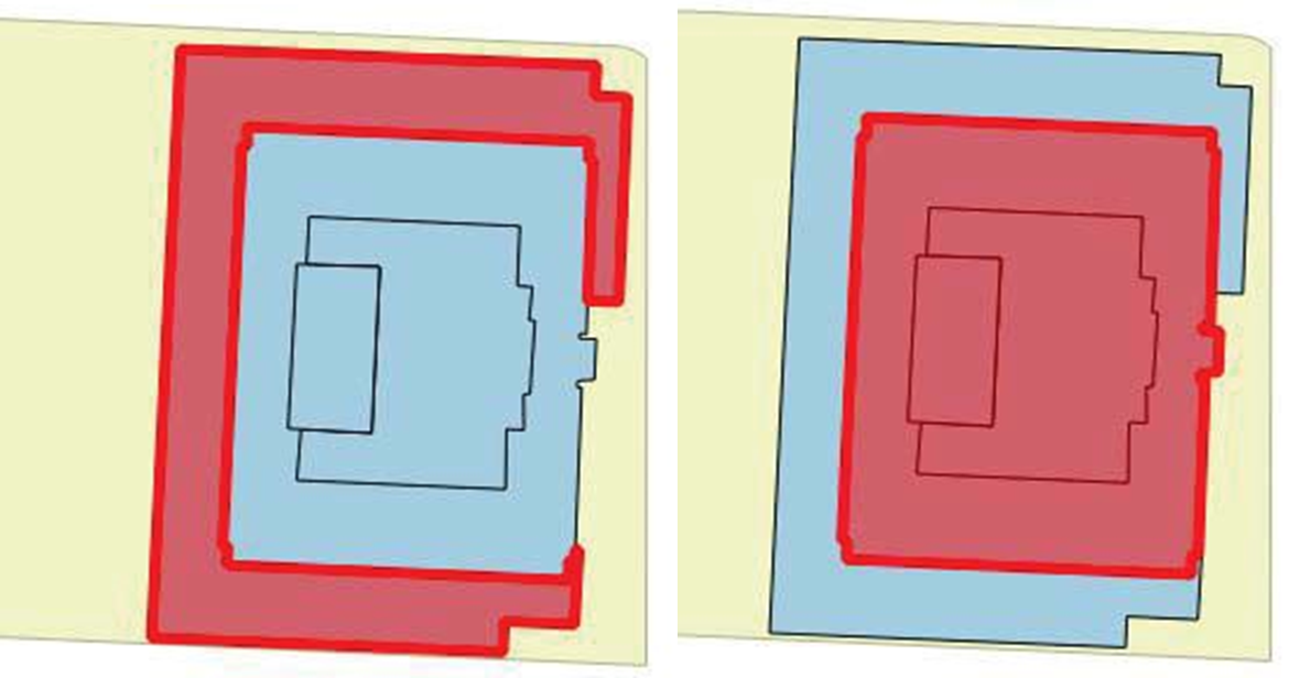
Figure E-1: Overlapping Building Polygons
Text version
A figure showing overlapping building polygons.
In addition to the footprint area and location of a building, information such as total use area and residential building type is required from the assessment records. Because there is typically no link between the building polygons and these records, another identifier must be used. The GIS address files would logically be the most suitable. However addresses can sometimes be problematic.
There are three types of addresses: Parcel Address, Suite Address, and Building Address. Unfortunately, not all buildings have addresses; many cover multiple parcels, and the assessment records do not correspond to the actual address in many cases. Exhibit E-2 is an example of a property that illustrates these issues.
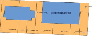
Figure E-2: Building, Parcel, Address and Assessment Record Issues
Text version
Figure showing the building, parcel, address and assessment record Issues
In the example in Figure E-2: One building does not have any address points. The building on the right has 146 address points (145 in the centre at the same spot). This includes suites and multiple building addresses. In the assessment records, all eight of the parcels shown have the address 395, 7 Street SW, the parcel address in the top right corner. All eight parcels also have the same roll number in the assessment records. That roll number has 992 records: a set of 124 for each parcel with the same details except for the parcel ID. All 992 records have building totals for office, retail, and storage space.
To avoid the known issues with building polygons and addressing, and to align the GIS inventory with the assessment records, a parcel-based approach is recommended. The parcel ID is a reliable link to the assessment records. The following (simplified) steps were employed to create a new inventory base:
All parcels in the assessment records with the same roll number are merged into one shape.
If the parcel contains multiple roll numbers, the space areas are summed. For residential condominiums, the number of records is counted as the number of units. The assessment records are then reduced to one record for each parcel or grouping of parcels with a single unique parcel identification number. The building footprint area is then calculated as a function of combined parcel coverage.
There are some instances of multiple buildings on a single parcel or group of combined parcels. Therefore, the building classification must be based on the predominant use and type. Similarly, the elevation is considered at the centroid of the parcel. This is slightly less precise in some cases but consistent with the judgments required to choose a classification when there is variation in use and elevation within individual buildings.
Having an inventory that reflects the data provided in the assessment records is of great importance because of the required estimates for indirect costs to businesses and households. Direct damage caused by flooding impacts the main and below-grade floors, while upper floors will incur other losses depending on the extent of the damage. This requires two inventory records for each multi-storey building, one relating to the main floor and the other for upper floors.
A residential unit count is also required to determine the number of impacted households. In the case of condominium multi-family, each unit will have an assessment record that can be counted as a unit. Rental buildings normally only have one record and when a unit count is not indicated or otherwise determined, the total living space is divided by an average unit size of 75 m2 to determine the approximate number of units.
J.1.3. Building Classification
Several internet tools can be used to assist in the identification and classification of a large number of records. Municipal mapping applications can be used to reconcile parcel and address information. Google Earth Pro’s Street View can be employed to determine the main floor use. Internet searches of addresses can be relied on to identify uses that are not clear from the street view. To facilitate the data entry related to building classification and estimated main floor elevation, IBI Group has developed a special application for use within Google Earth Pro. The GIS inventory was converted into a KML file with a field containing HTML code that allowed for data entry from the Google Earth interface. A user can then click on a particular parcel and enter the building classification, type, main floor elevation, presence of basement or underground parking, and other notes. Exhibit E-3 illustrates a screenshot of this tool in use.
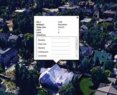
Figure E-3. GE Tool in Use
Text version
The figure is a screen capture of a tool used to edit building data using Google Earth.
Appendix 10 – Data Capture Forms – RESIDENTIAL
Occupants of these units can be recruited for participation in the survey with a letter from the relevant local authority explaining the nature and purpose of the data collection effort. Interviewers should follow up on the recruitment letter with personal visits or telephone calls to establish appointments for the data collection (IBI Group & ECOS Engineering Services Ltd., 1982). Flood assessors gather detailed damage cost estimates following a flood disaster and could be consulted to obtain damage estimates for given flood depths.
Data may be collected via a small team of well-trained interviewers. Interviewers should use computer-aided data capture to acquire and record structure and contents data. Interviewers should also be equipped with laser distance measuring devices to measure and record structure and contents dimensions. Interviewers should record information regarding:
- Single unit building floor area or multi-unit apartment floor area;
- Exterior finish materials and proportions;
- Foundation type: slab on grade (basement, pile, solid wall, pier/post, crawlspace, or fill
- Construction type: wood, steel, concrete, masonry or mobile home
- Quality of structure: below average, average, above average, or custom
- Building age
- Elevation from grade to top of first floor at entry;
- Individual room names, dimensions and location (storey) within the dwelling unit;
- Individual room, floor and wall finishes and areas;
- Dimensions of closets and storage shelving or storage units;
- The number, location, dimensions, and quality/value of all appreciable value content items located on the basement level, main floor level, in the garage, and outside at grade; and
- When recording data following an actual event, interviewers should also collect information on:
- Duration of flooding, short duration, long duration, extra long duration
- Warning time, less than 8 hours, greater than 8 hours
- Water quality
| Category of Water | Description |
|---|---|
| Major clean/grey (IICRC Category 2) | Water contains significant contamination and can contain potentially unsafe levels of microorganisms or nutrients for microorganisms, as well as other organic or inorganic matter: commonly discharge from washing machines, dishwashers or toilet overflows (not including faeces). |
| Minor black (IICRC category 3) | Water is grossly contaminated: As ‘Major clean/grey’, but includes sewage backflow scenarios from an internal source where water may contain faeces, urine and other waste through toilet discharge system. |
| Major flood/storm (IICRC category 3) | Water is grossly contaminated: This is the most common category for a typical fluvial, surface water or coastal flood scenario. Water may contain: organic matter, pesticides, heavy metals or toxic organic substances. |
| Major Flood including sewage (IICRC category 3) | Water is grossly contaminated: As 'Major flood/storm', but with the inclusion of animal and human waste materials. |
| Major Flood 'Contaminated' (IICRC Special situations) | Water may contain regulated hazardous waste (as per Technical Guidance WM2), including (but not limited to): asbestos, heavy metals, pesticides, solvents, caustic chemicals etc. |
The contents inventory should be aided by reference to a catalogue containing a list of furnishings and other content items commonly found in Canadian residences (Table J-2). Interviewers should also manually enter information on unusual or rare items not found in the common inventory catalogue.
Interviewers should assess each item of the contents to determine the depth of flooding at which significant damage would commence (the “significant level”), and the level at which the item would be completely inundated. Additionally, the interviewers should evaluate the quality and price range for each item of the contents based on visual assessment, reference to the catalogue, and discussion with the occupant. In some cases, content items of unusual quality or value are identified, which are not well represented by standard price ranges. In these cases, multiple quantities of the item should be recorded to approximate the estimated actual value of the item. For any unusual circumstances, the interviewers should record comments for later evaluation in the office. Many smaller items of minor value may be excluded from the contents inventory.
Any content item identified in the residential inventories is assumed to be destroyed once the depth of flooding exceeds the item’s significant level. It is possible for some non-permeable flood affected contents to be salvaged if their exposure to floodwater is limited to a number of hours. However, there is often insufficient capacity in the remediation industry to accommodate the large demand associated with large flood events and the costs associated with remediation often exceed the value of the item itself. Furthermore, some household materials are likely to become contaminated with mold following a flood.
For some items, such as storage shelving, bookcases, clothing closets, and refrigerators, content values may be estimated using stock prices, as in Exhibit J-2. An allowance for contents, such as books, clothing, etc. should be added to the value. Furthermore, for items with considerable vertical dimensions, such as clothing closets, it is assumed that damage commences at the item’s significant level and increases in proportion to the flood depth above the significant level.
The values assigned to residential contents should represent estimates of their current replacement cost. No attempt should be made to depreciate the value of these items; the current replacement cost estimates are intended to capture the totality of economic damage assuming that all of the damaged contents will be replaced with similar quantities and sizes of like quality.
The resulting structural and content inventory data should be prepared for office analysis using relational database and spreadsheet software.
Exhibit J-1A – Residential Data Capture Form - Building Structure
| Confidential flood damage survey estimate/ estimation confidentielle des dommages causés par les inondations | ||||||
| Inspector: | Date : | Time : | ||||
| Name: | Areas Inspected | Exterior only | Exterior & Interior | |||
| Home information | ||||||
| Address: Unit# Bldg# Street Name City |
||||||
| Building Contact ph: | Number of Residential Units : | Building Age | ||||
Type of Construction:
|
Exterior Finish*(%)
|
Primary Occupancy
|
||||
Building Elevation / Élévation du bâtiment, Height (m): (enter measured value of exterior grade to first floor – in metres to single decimal) |
||||||
Basement
|
Number of Stories:
|
Quality of Construction
|
Building Footprint / dimension du bâtiment (values in metres to single decimal value) Length (m): Width (m): Total Area (Sq m): |
|||
Page _______ of _________
Exhibit J-1B - Residential Data Capture Form - NonStructural Components
| Inspection: | |||||||||||||||||||||
|---|---|---|---|---|---|---|---|---|---|---|---|---|---|---|---|---|---|---|---|---|---|
| Inspector ID: | Inspection Date: | Time: | |||||||||||||||||||
| Interior: Household room information | |||||||||||||||||||||
| For each room complete the following details in the table below: | |||||||||||||||||||||
| Room Name | (enter description) | ||||||||||||||||||||
| Level: (in house) | Level 0 (Basement), Level 1 (First Floor, main living level), Level 2 (Second Floor), Level 9 (Other) | ||||||||||||||||||||
| Room Dimensions | (values in metres to single decimal value) | ||||||||||||||||||||
| Floor Surface: | Concrete (R), Ceramic Tile (CT), Vinyl/Laminate (VL), Wood (W), Carpet (C), Cork (K), or Other (O) | ||||||||||||||||||||
| Wall Surface: | Finished or Unfinished | ||||||||||||||||||||
| Closet Length: | (enter summed values in metres to single decimal value) | ||||||||||||||||||||
| Room Name | Room # | Level | Length (m) |
Width (m) |
Floor Surface | Wall Surface | Closet Lengths (total m) |
||||||||||||||
| . | . | . | |||||||||||||||||||
| . | . | . | |||||||||||||||||||
| . | . | . | |||||||||||||||||||
| . | . | . | |||||||||||||||||||
| . | . | . | |||||||||||||||||||
| . | . | . | |||||||||||||||||||
| . | . | . | |||||||||||||||||||
| . | . | . | |||||||||||||||||||
| . | . | . | |||||||||||||||||||
| . | . | . | |||||||||||||||||||
| . | . | . | |||||||||||||||||||
| . | . | . | |||||||||||||||||||
Page _______ of _________
Exhibit J-1C - Residential Data Capture Form - Building Contents
| Inventory of Contents for Rooms | |||||||||||||||
| Inspector ID: | Inspection Date: | Time: | |||||||||||||
|---|---|---|---|---|---|---|---|---|---|---|---|---|---|---|---|
| # | Item Name or Description | Level | Room # | # of Items | Cost Range (Low-Mid-High) | Critical Height* (m) | Top Height | ||||||||
| . | . | ||||||||||||||
| . | . | ||||||||||||||
| . | . | ||||||||||||||
| . | . | ||||||||||||||
| . | . | ||||||||||||||
| . | . | ||||||||||||||
| . | . | ||||||||||||||
| . | . | ||||||||||||||
| . | . | ||||||||||||||
| . | . | ||||||||||||||
| . | . | ||||||||||||||
| . | . | ||||||||||||||
| . | . | ||||||||||||||
| . | . | ||||||||||||||
*critical height is the height of the item at which significant damage would occur from floodwaters
Page _______ of ________
Post Flood Data Collection
After a flood has occurred, a post-flood building assessment checklist may be filled out to help identify flood levels in the building, submerged contents, safe access to the building etc. A post-flood assessment checklist is included.
Exhibit J-4 – Post Flood Assessment Form
| Rapid Damage Assessment Form (Post-Flood Event) Formulaire d'évaluation rapide des dommages (événement postérieur à l'inondation) |
||||||||||
|---|---|---|---|---|---|---|---|---|---|---|
| Inspector : | Date: 20_____ / ________ / _______ Y/A M/M D/J |
|||||||||
| Areas Inspected: | ☐ Exterior only | ☐ Exterior & Interior | ||||||||
| Home information | ||||||||||
| Address / Adresse: | ||||||||||
| Owner / Propriétaire | # of Residential Units: | |||||||||
| Exterior | ||||||||||
Type of Construction
|
Exterior Finish
|
Type of building:
|
||||||||
| Building Elevation / Élévation du bâtiment Height (m): ________________ (exterior grade to first floor / du rez-de-chaussée au rez-de-chaussée) |
||||||||||
Basement
|
Number of Stories :
|
Quality of Construction/ Qualité de de la construction
|
Building Footprint / Empreinte du bâtiment (values in metres to single decimal value)
|
|||||||
| Flood information | ||||||||||
| Initial Assessment of Damages: | ||||||||||
| Water Infiltration Levels: ☐ Basement(m) ☐ First Floor e (m): Lenght of Flooding (days)): | ||||||||||
Photos:
|
||||||||||
| Initial damage assessment | ||||||||||
| Foundation/basement | $ | |||||||||
| Structural damage/ wall, floor, ceiling & insulation | $ | |||||||||
| Heating System | $ | |||||||||
| Plumbing | $ | |||||||||
| Electrical & appliances | $ | |||||||||
| Initial assessment of damages: |
||||||||||
| Evaluation – exterior | ||||||||||
| Investigate the exterior building and area for the conditions below: |
||||||||||
| Minor/None | Moderate | Severe | Estimated Structure Damage
|
|||||||
| Collapse, partial collapse or building off foundation | ☐ | ☐ | ☐ | |||||||
| Building or story leaning/out of plumb | ☐ | ☐ | ☐ | |||||||
| Falling hazards (e.g. chimney, parapet, etc.) | ☐ | ☐ | ☐ | |||||||
| Slope failure, scour, erosion | ☐ | ☐ | ☐ | |||||||
| Damaged/Submerged fixtures or services (electric/gas) | ☐ | ☐ | ☐ | |||||||
| Proximity risks / other (specify) | ☐ | ☐ | ☐ | |||||||
| Other (specify) | ☐ | ☐ | ☐ | |||||||
| Posting Status: | ||||||||||
| ☐ Inspected (Green) | ☐ Restricted Use (Yellow) | ☐ Unsafe (Red) | ||||||||
| Add comments, including any of there are any restrictions to entry |
||||||||||
| Follow-up required: | Yes | No | Additional Comments: | |||||||
| Gas | ☐ | ☐ | ||||||||
| Electric | ☐ | ☐ | ||||||||
| Structural | ☐ | ☐ | ||||||||
| Plumbing | ☐ | ☐ | ||||||||
| Debris Removal | ☐ | ☐ | ||||||||
| Other | ☐ | ☐ | ||||||||
| Health: | ||||||||||
| Power Supply: Has the power been turned off? | ☐ Yes | ☐ No | How Long? | |||||||
| Were any foods affected by the loss of power? | ☐ Yes | ☐ No | Value? | |||||||
| Waste Water Disposal | ☐ Municipal | ☐ Private | ||||||||
| Did the septic system/sewer back up into the residence? | ☐ Yes | ☐ No | ||||||||
| Water supply | ||||||||||
| ☐ Drilled ☐ Municipal ☐ Other: | ||||||||||
| Was the water supply impacted by the flood? | ☐ Yes | ☐ No | ||||||||
| Sampling bottles left with resident? | ☐ Yes | ☐ No | ||||||||
| Food Supply: Were any foods affected by flood water? | ☐ Yes | ☐ No | ||||||||
| Indoor flood damaged areas | ||||||||||
| Walls: | ||||||||||
| Floors : | ||||||||||
| Furniture: | ||||||||||
| Health-Related Observations and Comments: |
||||||||||
| Additional Conditions Observed Requiring Attention: |
||||||||||
| Interior – contents | ||||||||||
| Address: | ||||||||||
| Unit # | Bldg # | Street Name and Type | City | |||||||
| Inspector ID: | Inspection Date: | Time: | ||||||||
| For each damaged item, enter the following details in the table below: Room Name: (enter description) Level: (in house) Level 0 (Basement), Level 1 (First Floor, main living level), Level 2 (Second Floor), Level 9 (Other) Item / Description: (enter description) Cost Range:enter estimated cost of item (refer to Exhibit F-2) for common household items Damage Estimate: put a checkmark in the appropriate column which represents the estimation of damage Salvageable: Yes (Y), the item can be cleaned and repaired, No (N) the item is not repairable |
||||||||||
| Item | Room | Level | Item / Description | Cost Range (Low-Mid-High) |
Damage Estimate | Salvageable | ||||
| 1 - 10 % | 11 - 30% | 31 - 60% | 61 - 99% | 100% | Y / N | |||||
| Address: | ||||||||||
| Owner/Propriétaire: | Tel: | ☐ Basement | Electrical Meter Numbe | |||||||
| Electrical | ||||||||||
| Affected Areas | ☐ Basement | ☐ Ground Floor | ||||||||
| ☐ Garage | ☐ Other | |||||||||
| Service Disconnected | ☐ Yes | Approximate Depth of Water (m): | ||||||||
| ☐ No | ||||||||||
| Electrical Items That Need to Be Replaced | ||||||||||
| Electrical contractor | ||||||||||
| ☐ Electrical Panel (incl. circuit breakers or fuses) | ☐ Electrical Conductors or Cables | |||||||||
| ☐ Electric Meter Socket | ☐ Sump Pump | |||||||||
| ☐ Domestic Hot Water Heater | ☐ Electrical Wiring Devices | |||||||||
| ☐ Electric | ☐ Oil | ☐ Gas | ☐ Switches | ☐ Réceptacle | ||||||
| ☐ Owner | ☐ Rental | ☐ Thermostats | ||||||||
| ☐ Furnace Burner, Blower Motor or Ignition Transformer | ☐ Electric Baseboard Heaters | |||||||||
| ☐ Electric Furnace | ☐ Lighting Fixtures | |||||||||
| ☐ Disconnect Switches | ☐ Electrical Splice Connectors | |||||||||
| ☐ Well Pump | ☐ Mast, Clevis, weatherhead | |||||||||
| ☐ Other (Provide List Below) | ☐ Electric Appliances (Provide List Below) | |||||||||
| Additional Conditions Observed Requiring Attention: |
||||||||||
| Inspector: | Date: | |||||||||
| Address: | ||||||||||
| Owner: | Tel: | Electrical Meter Number: | ||||||||
| Environment | ||||||||||
| Site accessibility acceptable? | ☐ Yes ☐ No | Comment: | ||||||||
| Contamination: | ☐ Yes ☐ No | Comment: | ||||||||
| Source identified | ☐ Yes ☐ No | |||||||||
| Water Supply | ☐ Drilled | ☐ Sand Point | ||||||||
| ☐ Municipal | ☐ Unknown Source | |||||||||
| Impact/Potential for impact | ☐ Yes ☐ No | |||||||||
| Sample bottle provided? | ☐ Yes ☐ No | |||||||||
| Watercourse | ||||||||||
| Name: | ||||||||||
| Impact/Potential for impact | ☐ Yes ☐ No | |||||||||
| If yes, type of impact | ||||||||||
| Additional Conditions: |
||||||||||
| GPS: |
||||||||||
| Inspector: | Date: | |||||||||
Appendix 11 – Data capture forms – Non- Residential
Data regarding potential damage to commercial buildings may be collected via a survey questionnaire issued to proprietors or store managers regarding:
- The value of their inventories;
- The percentage damageable at each unit depth of flooding;
- Possibilities of salvage;
- Values of equipment and furniture; and
- Structural characteristics of the building including, but not limited to, heating and air conditioning systems and electric panels.
Essentially, the objective of the survey is to obtain information regarding damages to inventory, equipment, raw materials, and structures, as well as clean-up costs such that stage-damage curves may be constructed from the information. To guide the process, a sample questionnaire is included in Appendix 17.
If cooperation is not received from proprietors and store managers, field personnel can obtain a rough estimate of the total inventory by sampling the premises. In this case, shelves, racks, counters, and display cabinets should be measured and the value of goods found in selected sample areas within each type of display or storage unit should be recorded. The total value of goods in the building can be estimated based on the average value per unit of storage area sampled. For example, the average value of goods per unit length of shelving can be applied over the entire length of shelving in the building to estimate a total value.
Where the study scope permits and where commercial damages are an important component, a field survey of commercial establishments is recommended. However, where budgets preclude detailed damage surveys, commercial stage-damage curves can be developed based on the guidelines provided in IBI Group & Golder Associates (2015). Commercial damage curves are presented in Appendix 13.
The office/retail category generally exhibits a higher level of finishing, carpeting, wallboard, higher level of ceiling finishes, more doors and partitions, etc.
The industrial/warehouse category typically contains a small portion of office and is generally characterized by a lack of partitions and a very low ratio of finished to unfinished interior space.
The hotel/motel category typically has a combination of suites and function rooms including banquet halls, restaurants and lounges on the lower levels with a medium to high level grade of interior finish.
The institutional category covers a variety of buildings including schools, libraries and other purpose-built public facilities with durable interior and exterior finishes and generally more expensive construction
Commercial property flood damage estimate study (Confidential)
Address:
Business Name:
Business Type:
Contact:
Flood Zone:
Interviewer:
Date:
Telephone:
- Construction Type: _____
- Average Exterior Dimensions, L x W: ____
- Interior Construction:
| Level 0-2 | Display | Storage | Manufacturer | Office | Length | Width | Height | Material | |
|---|---|---|---|---|---|---|---|---|---|
| Wall | Floor | ||||||||
- Estimated Total Value of Inventory: $___
- Depth/Damage Table for Contents:
| Flood Depth | Level 0 (%) | Level 1 (%) | Level 2 (%) | |
|---|---|---|---|---|
| 0.15 m | .5 ft | |||
| 0.3 m | 1 ft | |||
| 0.6 m | 2 ft | |||
| 0.9 m | 3 ft | |||
| 1.2 m | 4 ft | |||
| 1.5 m | 5 ft | |||
| 1.8 m | 6 ft | |||
| 2.4 m | 8 ft | |||
| 3.0 m | 10 ft | |||
- % of Total Inventory
Located on Level: ___% + ___% +___ % = 100%
- % of Total Inventory Salvageable: ___%
- Inventory of Contents for Rooms:
| Item | Number | Significant Level | Cost 1-3 | Age Years |
|---|---|---|---|---|
| Furnace (Fuel Type: _) | ||||
| Water Heater | ||||
| Electrical Panel | ||||
| Air Conditioner | ||||
- Employee Information:
| Type of Employment | Number | Average Wages |
|---|---|---|
| Full Time | $____ /week | |
| Part Time (< 20 hours) | $ ____/hour |
- Flood Experience:
| Ground Floor | Basement | Number of Employees Laid Off | $ Lost Business | Post-Flood Scale Income Made Up Lost Business | |||
|---|---|---|---|---|---|---|---|
| Water Level (m) | % Damage | Water Level (m) | % Damage | Salaried | Hourly | ||
- Include comments and additional information:
Appendix 12 – Stage Damage Curves and Values – Residential
Alberta:
Developed for Government of Alberta ESRD – Resilience and Mitigation by IBI Group, 2015. Provincial Flood Damage Assessment Study. Stage-damage curves were developed for Calgary region and the report includes recommended provincial adjustment indexes
IBI Group. "Golder Associates, 2015. “Provincial Flood Damage Assessment Study.” Government of Alberta.
Ontario:
Developed in 1985, 34 synthetic stage-damage curves were created from seven communities in southern Ontario.
Paragon Engineering Limited, Environment Canada, Ontario Ministry of Natural Resources (1985) Development of flood depth-damage curves for residential Homes in Ontario—Vol I—Technical Report.
Available online: Government of Canada, Federal Science Library
Appendix 13 – Stage Damage Curves and values - Non-Residential*
City of Calgary, 2014 (Damages for underground parking is $215 /m)
The presented commercial structural damage curves have been based on inundation with a two to three day recession period. They assume virtually no damage to walls due to hydrostatic pressure as water is anticipated to leak in around window sashes, doors and other openings. Further, the curves assume no damage to structures as a result of blocks of ice (associated with ice jam flooding) contacting exterior walls.
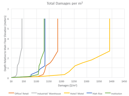
Figure P-1: Non-residential structure
Text version
Graph showing total damage per square metre for a non-residential structure.
| Relative Depth (m) | Non-residential structure | ||||
|---|---|---|---|---|---|
| S1 Office/ Retail |
S2 Industrial/ Warehouse |
S3 Hotel/ Motel |
S4 High Rise |
S5 Institution |
|
| 0 | $0 | $0 | $0 | $0 | $0 |
| 0.1 | $105 | $16 | $113 | $79 | $68 |
| 0.3 | $127 | $21 | $212 | $79 | $107 |
| 0.6 | $132 | $23 | $230 | $105 | $108 |
| 0.9 | $135 | $23 | $242 | $116 | $109 |
| 1.2 | $138 | $24 | $254 | $134 | $110 |
| 1.5 | $155 | $30 | $284 | $134 | $115 |
| 1.8 | $164 | $31 | $320 | $134 | $117 |
| 2.7 | $185 | $38 | $391 | $134 | $130 |
| 3 | $185 | $42 | $391 | $134 | $130 |
| 5 | $185 | $42 | $391 | $134 | $130 |
| 6 | $185 | $42 | $391 | $134 | $130 |
| Code | Non-residential Contents | Relative Depth (m) | |||||||||||
|---|---|---|---|---|---|---|---|---|---|---|---|---|---|
| 0 | 0.15 | 0.3 | 0.6 | 0.9 | 1.2 | 1.5 | 1.8 | 2.1 | 2.4 | 2.7 | 3 | ||
| A1 | General Office | 0 | 121 | 127 | 219 | 380 | 380 | 380 | 380 | 380 | 380 | 381 | 381 |
| B1 | Medical | 0 | 150 | 450 | 900 | 1350 | 1380 | 1425 | 1500 | 1500 | 1500 | 1500 | 1500 |
| C1 | Shoes | 0 | 200 | 600 | 729 | 984 | 1100 | 1121 | 1159 | 1189 | 1219 | 1219 | 1219 |
| C2 | Clothing | 0 | 187 | 385 | 572 | 1314 | 1425 | 1705 | 1862 | 1862 | 1862 | 1862 | 1862 |
| C3 | Stereos/ TV | 0 | 352 | 504 | 689 | 852 | 1139 | 1352 | 1467 | 1467 | 1467 | 1467 | 1467 |
| C4 | Paper Products | 0 | 96 | 183 | 366 | 557 | 740 | 810 | 906 | 906 | 906 | 906 | 906 |
| C5 | Hardware/ Carpet | 0 | 142 | 265 | 427 | 880 | 943 | 1005 | 1068 | 1130 | 1257 | 1257 | 1257 |
| C6 | Retail | 0 | 209 | 408 | 636 | 844 | 1072 | 1252 | 1366 | 1366 | 1366 | 1366 | 1366 |
| C7 | Misc Retail | 0 | 182 | 349 | 512 | 782 | 919 | 1026 | 1103 | 1115 | 1134 | 1134 | 1134 |
| D1 | Furniture/ Appliances | 0 | 138 | 198 | 306 | 345 | 376 | 408 | 439 | 439 | 439 | 439 | 439 |
| E1 | Groceries | 0 | 148 | 270 | 410 | 531 | 616 | 616 | 616 | 616 | 616 | 616 | 616 |
| F1 | Drugs | 0 | 50 | 350 | 505 | 610 | 715 | 820 | 897 | 897 | 897 | 897 | 897 |
| G1 | Auto | 0 | 46 | 254 | 462 | 878 | 982 | 1005 | 1005 | 1005 | 1005 | 1005 | 1005 |
| H1 | Hotels | 0 | 20 | 39 | 52 | 65 | 104 | 131 | 144 | 144 | 144 | 144 | 144 |
| I1 | Restaurant | 0 | 72 | 257 | 434 | 442 | 452 | 452 | 452 | 452 | 452 | 452 | 452 |
| J1 | Personal Services | 0 | 37 | 74 | 167 | 260 | 278 | 408 | 687 | 696 | 705 | 705 | 705 |
| K1 | Financial | 0 | 121 | 127 | 219 | 380 | 380 | 380 | 380 | 380 | 380 | 380 | 380 |
| L1 | Warehouse/ Industrial | 0 | 173 | 433 | 635 | 1011 | 1155 | 1184 | 1242 | 1285 | 1328 | 1357 | 1386 |
| M1 | Theatres | 0 | 0 | 0 | 68 | 68 | 68 | 68 | 68 | 68 | 68 | 344 | 621 |
| N1 | Institution | 0 | 59 | 119 | 312 | 446 | 475 | 475 | 475 | 475 | 475 | 475 | 475 |
| N2 | Hospital | 0 | 72 | 92 | 182 | 311 | 341 | 363 | 363 | 363 | 363 | 363 | 363 |
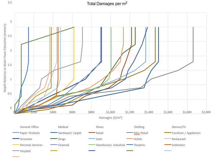
Figure P-2: Non-Residential Contents
Text version
Graph showing damage per square metre for the contents of a non-residential structure.
Appendix 14 – Sample Content and Prices
| Sample Content | LOW Mean 1 |
MEDIUM Mean 2 |
HIGH Mean 3 |
Mean All |
|---|---|---|---|---|
| Art / mirror on wall | $100 | $250 | $750 | $367 |
| BBQ | $210 | $433 | $1,119 | $567 |
| Bed head/foot board | $451 | $917 | $2,751 | $1,318 |
| Bed mattress | $651 | $1,196 | $2,265 | $1,342 |
| Bicycle | $223 | $450 | $2,962 | $1,131 |
| Bookcase linear metres | $702 | $1,493 | $2,511 | $421 |
| Camera / video | $133 | $257 | $933 | $420 |
| Camping gear set | $459 | $693 | $1,007 | $712 |
| Chest of drawers | $879 | $1,632 | $3,225 | $2,008 |
| Clothing closet linear metre | $1,402 | $2,625 | $5,240 | $3,089 |
| Clothing steamer | $153 | $153 | $153 | $153 |
| Coffee machine | $88 | $144 | $1,041 | $395 |
| Computer desktop | $574 | $851 | $1,330 | $906 |
| Computer laptop | $365 | $612 | $1,198 | $709 |
| Computer tablet | $204 | $391 | $724 | $431 |
| Cooktop / wall oven | $3,060 | $3,780 | $5,992 | $4,213 |
| Dining chair / table set | $558 | $1,257 | $3,085 | $1,582 |
| Dishwasher | $496 | $734 | $1,626 | $925 |
| Footstool / ottoman | $82 | $151 | $597 | $263 |
| Freezer | $993 | $1,311 | $1,908 | $1,388 |
| Furniture wall unit linear (m) | $1,402 | $2,625 | $5,240 | $3,089 |
| lawn mower / snow blower | $301 | $494 | $1,296 | $673 |
| Garden other power hand equipment | $89 | $145 | $320 | $180 |
| Iron & board | $106 | $106 | $106 | $106 |
| Kitchen equipment | $84 | $216 | $442 | $250 |
| Kitchen waste disposal | $193 | $193 | $193 | $193 |
| Lamp floor / table | $53 | $146 | $348 | $177 |
| Luggage set 3pc | $119 | $255 | $470 | $276 |
| Microwave | $105 | $168 | $372 | $209 |
| Musical instrument piano / organ | $2,000 | $5,000 | $10,000 | $5,667 |
| Musical instrument portable | $1,000 | $3,000 | $5,000 | $3,000 |
| Night stand | $156 | $398 | $966 | $491 |
| Occasional chair | $221 | $451 | $1,120 | $578 |
| Office chair | $119 | $220 | $555 | $288 |
| Office desk | $217 | $702 | $1,482 | $781 |
| Office paper shredder | $76 | $158 | $350 | $189 |
| Office printer | $79 | $142 | $344 | $182 |
| Outdoor patio set | $557 | $1,608 | $3,458 | $1,827 |
| Pool / games table | $304 | $935 | $2,895 | $1,321 |
| Refrigerator | $1,436 | $2,311 | $3,176 | $2,290 |
| Rug area <5 m2 | $226 | $562 | $951 | $579 |
| Rug area 10+m2 | $1,089 | $2,140 | $5,755 | $2,961 |
| Rug area 5-10 m2 | $349 | $739 | $1,711 | $925 |
| Sewing / serger machine | $168 | $347 | $946 | $487 |
| Sideboard | $912 | $1,729 | $3,444 | $1,982 |
| Sofa/love seat per position | $271 | $455 | $899 | $530 |
| Sound system equipment | $244 | $417 | $941 | $519 |
| Sound system headphones | $62 | $180 | $335 | $188 |
| Sound system speakers | $142 | $293 | $834 | $407 |
| Sports gear set | $767 | $767 | $767 | $767 |
| Storage shelving linear metres | $272 | $272 | $272 | $272 |
| Stove | $870 | $1,400 | $2,232 | $1,480 |
| Table accent / end | $139 | $295 | $954 | $443 |
| Table coffee | $182 | $359 | $858 | $452 |
| Telephone set | $83 | $83 | $83 | $83 |
| Television DVR/ streaming hub | $213 | $213 | $213 | $213 |
| Television set | $323 | $797 | $2,359 | $1,114 |
| Treadmill / elliptical | $546 | $1,532 | $2,873 | $1,619 |
| TV / media bench / cabinet | $226 | $763 | $2,437 | $1,093 |
| Vacuum portable | $162 | $335 | $563 | $348 |
| Warming drawer | $1,308 | $1,308 | $1,308 | $1,308 |
| Washer / dryer set | $1,199 | $1,738 | $2,572 | $1,816 |
| Weight machine | $641 | $1,452 | $3,720 | $1,873 |
| Window covering to floor | - | - | - | - |
| Window covering to sill | - | - | - | - |
| Wine rack number bottles | $10 | $19 | $38 | $22 |
| Workshop bench / table | $265 | $265 | $265 | $265 |
| Workshop power tools / equipment | $94 | $150 | $305 | $179 |
Table J-3: Price Suppliers (4,000 Individual Item Prices)
- Amber's Furniture
- Ashley Furniture Homestore
- Atlas Appliance Expert
- babies'R'us
- Bass Pro Shops
- Bed Bath Home
- BestBuy
- Birchwood Furniture Galleries
- Bombay Company
- Bondars Furniture
- Canada Mountain Bike Shop
- Canadian Tire
- Consumer Reports
- Costco
- Crate & Barrel
- Cricklewood Interiors
- Crossroads Furniture
- Gallery Dell
- Eisenberg's Fine Furniture
- Fitness Depot
- Furniture Depot
- Future Shop
- Giant Bicycles
- Hockey Plus
- Home Outfitters
- Hudson's Bay
- IKEA JYSK
- Lamps.com
- Lane Home Furnishings
- LaZboy Home Furnishings
- Leon's Furniture
- London Drugs Lowe's
- Major Appliances Inc.
- McArthur Fine Furniture
- Mountain Eqiupment Co-op
- Office Depot
- Pooltables.ca
- PotteryBarn
- Restoration Hardware
- Sears
- SleepCountry
- SportChek
- Staples
- Structube Furniture
- Target
- The Brick
- The Home Depot
- The Source
- Urban Barn
- Visions Electronics
Appendix 15 – Review of Building Classification Schemes and Photographic Examples of Building Classes
Housing types, building practices, and materials are relatively uniform across most of the country given the existence of the National Building Code. The obvious exceptions are the more temperate regions of British Columbia, where basements or extended foundations are not required, and the far north, where permafrost conditions can limit basement development and also influence specialty mechanical systems for larger buildings.
K. Evolution of Building Classification Schemes
The residential classification scheme employed in the Acres Limited (1968) Study categorized residential structures as either wood or brick with a further definition of three sub-categories for each of these. This system of classification conformed to a scheme devised by the Ontario Department of Municipal Affairs. A handbook was published by the Department which contained detailed descriptions and cross-sections of the type of homes found within each of the sub- categories, thus facilitating efficient and consistent field classification within the pilot study and subsequent studies employing the Acres methodology. The general elements of this scheme are presented in Table F-1.
Table F-1: Acres Residential Classification Scheme (Acres Limited, 1968)
| Class | Department of Municipal Affairs Designation | General Criteria |
|---|---|---|
| AW | D-7 to D-10 | Solid, architect-designed wooden structure. May be ultra-modern or older two-storey. High-class, solid construction and materials |
| BW | D-4 to D-6 | Double wall frame home. Typical of middle-class housing developments. Most wooden homes fall into this class |
| CW | D-1 to D-3 | Rough frame structure, thin walls. May have stucco or imitation brick coating. |
| Class | Department of Municipal Affairs Designation | General Criteria |
|---|---|---|
| AB | C-8 to C-10 | Mansion-like or ultra-modern appearance. Very high quality in construction and materials. |
| BB | C-6 to C-7 | Typical mass-produced ranch-style or two-storey home |
| CB | C-4 to C-5 | Cheap brick or concrete block bungalow. |
On the basis of the inventory undertaken for Fort McMurray, the Acres classification scheme was modified to reflect the particular nuances of the study area and furthermore, expanded to include several structural types not addressed within the Acres scheme (IBI Group & ECOS Engineering Services Ltd., 1982). These consisted of mobile homes, walk-up apartments and apartment towers. Three sub-categories were devised for each of the main categories, reflecting the quality and, to a lesser extent, size (m2) of the units (there is generally a strong correlation between the latter two factors).
The residential classification scheme devised for the Fort McMurray study is presented in Table F-2.
| Class | General Description |
|---|---|
| AW-1* AW-2 AW-3 | Typical custom constructed housing built, for the most part, during the 1970s architecturally designed with control of materials selection and consideration of increased insulation values, vapour seals, passive and active solar heating systems. Interior materials, finishes and general décor reflect an above average upgrading to· the personal requirements of the owner. These houses represent the high end in terms of real estate values. |
| BW-1 BW-2 BW-3 | Typical subdivision construction of the 1960s, constructed by the developer or builders from a selection of stock design plans in accordance with design guidelines for exterior materials control. Exterior materials are typically aluminum and wood siding, stucco and brick veneer. The size of the unit, style and lot size set the average real estate value. These houses have average insulation values and represent middle real estate values. |
| CW-1 CW-2 CW-3 | Typically constructed during the 1940s to 60s, units are of average design, less than average m2(<300), have a low level of insulation value, no vapour barrier or vapour seal and generally have exterior finishes of wood siding and stucco. Generally, these units are located in the core area have a high land to building value ratio and represent the lower end real estate values. Many units will have upgraded interior finishes. |
| D-1 | Mobile Home, Double Wide - Good Quality |
| D-2 | Mobile Home, Double Wide - Poor Quality |
| D-3 | Mobile Home, Single Wide - Good Quality |
| D-4 | Mobile Home, Single Wide - Poor Quality |
| MA | Apartment Towers |
| MW | Walk-Up Apartments, Row Townhouses |
* 1, 2, 3 denotes above average, average and below average quality within the A, B and C categories. This differentiation was later dropped for sampling purposes.
(IBI Group & ECOS Engineering Services Ltd., 1982)
For the Paragon Engineering Study of Ontario Depth-Damage Curves in 1985, a seven-fold classification system was adopted reflecting architectural structural types (Paragon Engineering Limited, 1985). It is illustrated in Table F-3.
| Group number | Group type | Categories included (from exhibit d-3b) | Sample size |
|---|---|---|---|
| 1 | 1 Storey with Basement | 1, 6, 11, 16, 21, 26 | 76 |
| 2 | 1 Storey no Basement | 2, 7, 12, 17, 22, 27 | 24 |
| 3 | 2 Storeys with Basement | 3, 8, 13, 18, 23, 28 | 99 |
| 4 | 2 Storeys no Basement | 4, 9, 14, 19, 24, 29 | 28 |
| 5 | Split-Level | 5, 10, 15, 20, 25, 30 | 26 |
| 6 | Townhouse | 31, 32, 33 | 19 |
| 7 | Mobile Home | 34 | 15 |
| TOTAL: 287 | |||
The residential classification scheme previously developed by Paragon Engineering Limited (1985) and employed by the consultant team in various Canadian studies was refined for the purposes of the Alberta Provincial Flood Damage Assessment Study of 2015. Residential structures are classified according to their construction techniques, size and quality and their number of stories. As property tax assessment data and GIS building footprint data are now readily available, this information was used to classify residential structures as single unit or low density unit types; medium density and high density. The residential classification scheme is summarized in Table F-4; photographs of typical residential structures of each type are depicted in Exhibit F-1A and B.
| Category Number | Style | Number of Storeys | Basement | Quality |
|---|---|---|---|---|
| 1 | Masonry | 1 | Y | Above |
| 2 | Masonry | 1 | N | Above |
| 3 | Masonry | 2 | Y | Above |
| 4 | Masonry | 2 | N | Above |
| 5 | Masonry | Split | --- | Above |
| 6 | Masonry | 1 | Y | Average |
| 7 | Masonry | 1 | N | Average |
| 8 | Masonry | 2 | Y | Average |
| 9 | Masonry | 2 | N | Average |
| 10 | Masonry | Split | --- | Average |
| 11 | Masonry | 1 | Y | Below |
| 12 | Masonry | 1 | N | Below |
| 13 | Masonry | 2 | Y | Below |
| 14 | Masonry | 2 | N | Below |
| 15 | Masonry | Split | --- | Below |
| 16 | Wood Frame | 1 | Y | Above |
| 17 | Wood Frame | 1 | N | Above |
| 18 | Wood Frame | 2 | Y | Above |
| 19 | Wood Frame | 2 | N | Above |
| 20 | Wood Frame | Split | --- | Above |
| 21 | Wood Frame | 1 | Y | Average |
| 22 | Wood Frame | 1 | N | Average |
| 23 | Wood Frame | 2 | Y | Average |
| 24 | Wood Frame | 2 | N | Average |
| 25 | Wood Frame | Split | --- | Average |
| 26 | Wood Frame | 1 | Y | Below |
| 27 | Wood Frame | 1 | N | Below |
| 28 | Wood Frame | 2 | Y | Below |
| 29 | Wood Frame | 2 | N | Below |
| 30 | Wood Frame | Split | --- | Below |
| 31 | Townhouse | --- | --- | Above |
| 32 | Townhouse | --- | --- | Average |
| 33 | Townhouse | --- | --- | Below |
| 34 | Mobile Home | --- | --- | --- |
* Y = Yes, N = No
(Paragon Engineering Limited, 1985)
| Class | Floor Area | General Description |
|---|---|---|
| AA-1 AA-2 |
372+ m2 (4,000+ ft2) Typical 456 m2 (4,903 ft2) |
Typically custom construction built during the 2000s, with superior architectural design and premium quality construction materials, finish materials and workmanship. These units typically include numerous large windows, extensive basement finishing, superior millwork, and built-in high-quality appliances. These very large dwelling units are few in number, and account for the highest reaches of the real estate price distribution, with an average value of $3,400,000.* |
| A-1 | 223 – 371 m2 (2,400 – 3,999 ft2) |
The A Class structures are relatively large, high-end homes typically featuring moderately high-quality construction materials and finishes. These units have good quality millwork and large window area ratios, and typically have most of the basement areas finished, and have attached garages. While much more numerous than the AA Class, the units represent a relatively small share of the total population of single dwelling units, reflective f their upper-middle price positioning, with an average value of $1,400,000.* |
| A-2 | Typical 266 m (2,858 ft2)2 |
|
| B-1 | 112 – 223 m2 (1,200 – 2,399 ft2) |
B Class units are generally the most numerous type of single dwelling units in Alberta municipalities. These average quality units were generally built from stock plans as tract or speculative housing for mid- market consumers, from the 1950s onward. These houses are typified by conventional design, and medium quality materials, finishes and workmanship, with some basement finishing and detached garages. They have an average value of $680,000.* |
| B-2 | Typical 163 m2 (1,754 ft2) |
|
| C-1 | <112 m2 (<1,200 ft2) |
The C Class units tend to be older housing stock in inner-city locations or tract starter housing in newer suburban locations. These houses are of average to below average quality in terms of design and construction materials, finishes and workmanship. Generally, units of this class located in the municipal core area have a high land to building value ratio as these structures are approaching functional and physical obsolescence. While C Class units represent the lower range of real estate values, many of these units have been upgraded by owners and feature average or better quality finishes in the renovated areas. They have an average value of $450,000.* |
| C-2 | Typical 88 m2 (947 ft2) |
|
| D | Typical 128 m2 (1,377 ft2) | D Class units are mobile homes, located on temporary foundations, and without basements. These units tend to reflect the lower range of real estate values. |
| MA | Typical 93 m2 (1,002 ft2) |
MA units are apartment units located in high-rise (5+ storey) structures. The high-rise apartment towers are typically of concrete and light steel frame construction, and have one or more levels of underground parking. |
| MW | Typical 65 m2 (704 ft2) | MW units are apartments located in low-rise (less than 5 storey) apartment structures. These structures are typically of wood construction and often have single level concrete parking structures underground. |
* Calgary assessed market values 2015.
| Class | Description |
|---|---|
| RES1 | Single Family Dwelling |
| RES2 | Mobile Home |
| RES3A | Duplex |
| RES3B | Triplex |
| RES3C | Row Housing, Multi-family garden apartment, rental townhouse |
| RES3D | Strata-Lot Residence |
| RES3E | Multi-family – apartment block (< 5 stories) |
| RES3F | Multi-Family – apartment, high rise (> 5 stories) |
| Alberta | HAZUS Codes | Floor Area (m2) | General Description | Stories | Quality Options |
|---|---|---|---|---|---|
| AA | RES1 | ~372 | Single-family dwelling with and without basement | 1,2 | Above, Custom |
| A | RES1 | 223-371 | Single-family dwelling with and without basement | 1,2,3,4 | Above, Average |
| B | RES1 | 112-223 | Single-family dwelling with and without basement | 1,2,3,4 | Above, Average, Below |
| C | RES1 | <112 | Single-family dwelling with and without basement | 1,2,3,4 | Above, Average, Below |
| D | RES2 | ~128 | Mobile Home | 1 | Above, Average, Below |
| E | RES3A, 3B | Duplex, Triplex, Row townhouse | 1,2,3* | Above, Average, Below | |
| MA | RES3D, 3F or 3F | high rise apartment | 2,3* | Above, Average, Below | |
| MW | RES3C | walk up apartment | 1,2* | Above, Average, Below |
*StatCan: Statistics Canada classification of building permit types
Exhibit F-1 - Typical Residential Classification Examples from Alberta Provincial Flood Damage Assessment Study
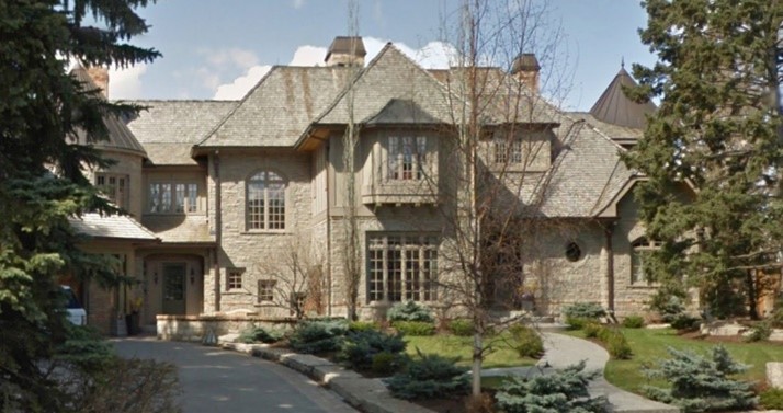
Code: RAA
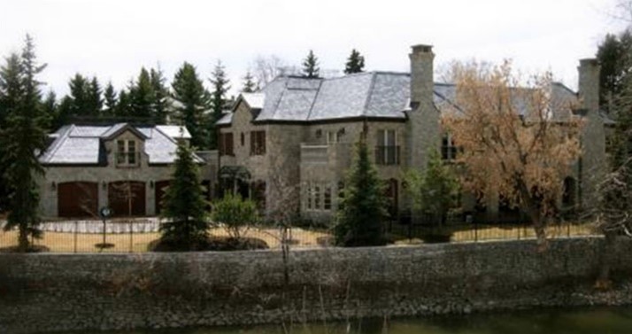
Code: RAA
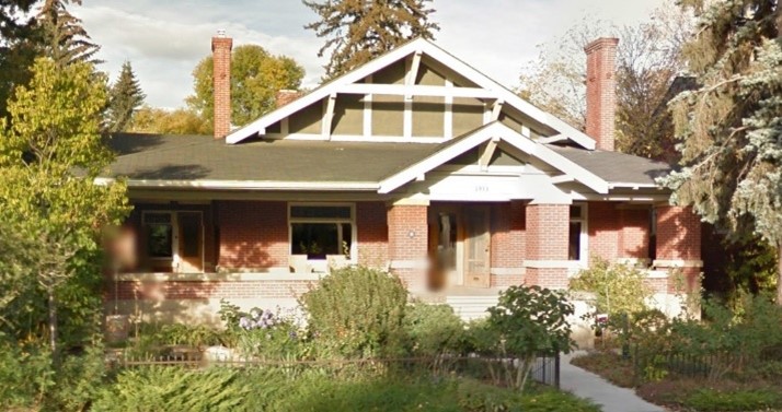
Code: RA
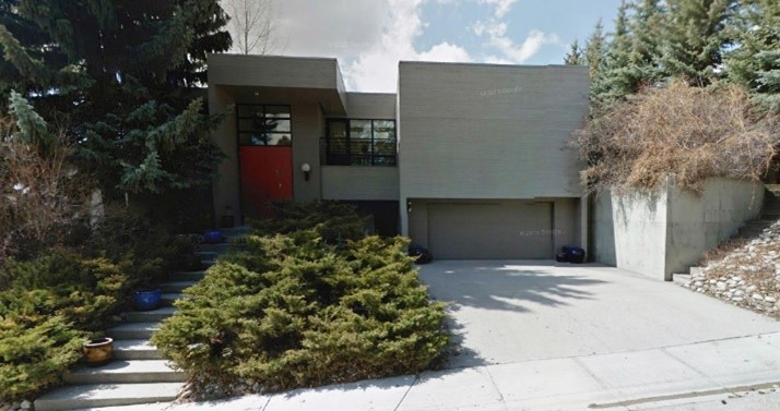
Code: RA
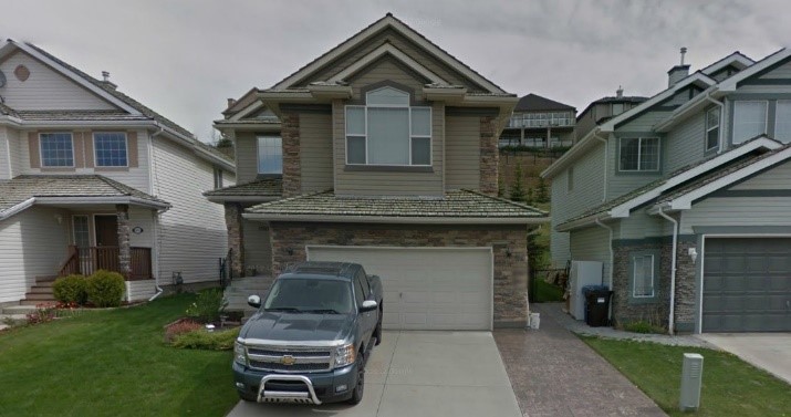
Code: RA
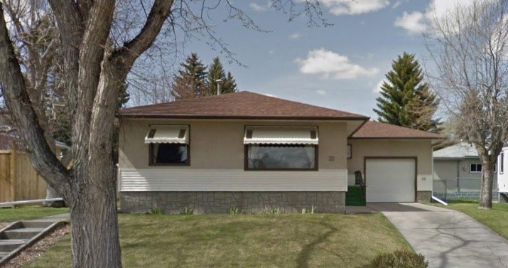
Code: RB
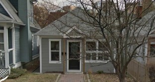
Code: RB

Code: RC
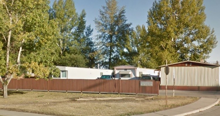
Code: RD
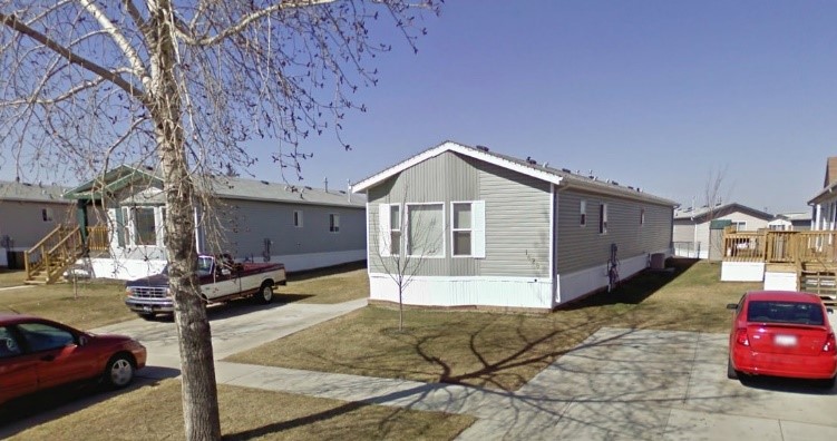
Code: RD
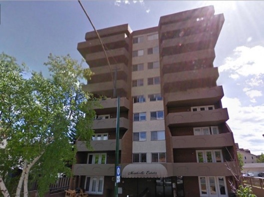
Code: RMA
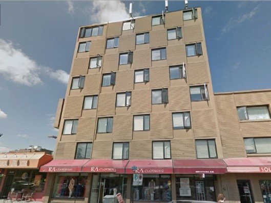
Code: RMA
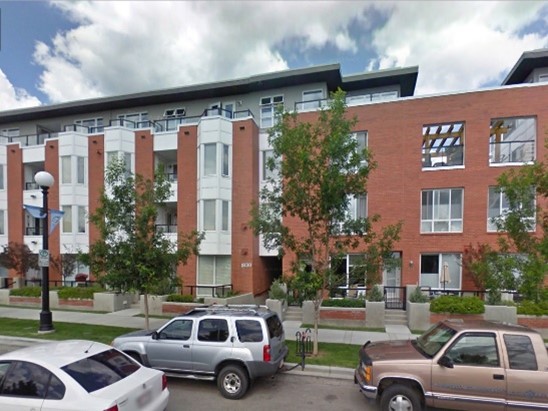
Code: RMW
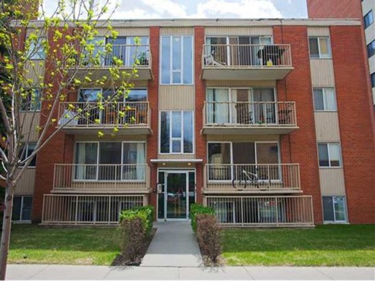
Code: RMW
| Class | HAZUS Code | General Description | Average m2 |
|---|---|---|---|
| A1 | COM4 | General Office | 1107 |
| B2 | COM7 | Medical | 386 |
| C1 | COM1 | Shoes | 138 |
| C2 | COM1 | Clothing | 427 |
| C3 | COM1 | Stereos/ TV/ Electronics | 385 |
| C4 | COM2 | Paper Products | 225 |
| C5 | COM4 | Hardware/Carpet | 594 |
| C6 | COM1 | Misc. Retail | 463 |
| D1 | COM1 | Furniture/Appliances | 336 |
| E1 | COM1 | Groceries | 1023 |
| F1 | COM7 | Drugs | 926 |
| G1 | COM1 | Auto | 385 |
| H1 | RES4 | Hotels | 661 |
| I1 | COM8 | Restaurants | 438 |
| J1 | COM4 | Personal Service | 163 |
| K1 | COM3 | Financial | 421 |
| L1 | IND1 | Warehouse/Industrial | 637 |
| M1 | COM8 | Theatres | 901 |
| N1 | RES5 | Other/Institutional | 1366 |
| O1 | COM6 | Hospital | 7613 |
| P1 | GOV2 | Police | - |
| Q1 | IND3 | Industrial - Food/Drugs/Chemicals | - |
| R1 | IND4 | Industrial - Metals/minerals processing | - |
| S1 | IND5 | Industrial - High technology | - |
| T1 | REL1 | Church/NonProfit | - |
| U1 | EDU1 | Grade School | - |
| V1 | EDU2 | College/University | - |
| X1 | GOV1 | General services (Government) | - |
| Y1 | GOV2 | Emergency response (Government) | - |
(IBI Group & Golder Associates, 2015)
| Class | HAZUS Code | General Descriptio |
|---|---|---|
| W1 | AGR1 | Agriculture - Crops |
| W1 | AGR1 | Agriculture – Livestock |
| W1 | AGR1 | Agriculture – Buildings and Equipment |
Exhibit F-2 - Commercial Classification Examples from Alberta Provincial Flood Damage Assessment Study


Appendix 16 – Residential Property External Damages
P.1. Residential Property External Damages
Referring to the residential classification scheme presented in Exhibit F-1 of Appendix 15, nominal values of $2,500; $5,000; $7,500; and $15,000 may be attributed to properties classified as C, B, A, and AA to account for landscaping and yard clean-up costs following a flood (IBI Group & Golder Associates, 2015). For buildings classified as MA or MW, a value of $15,000 per building may be applied (IBI Group & Golder Associates, 2015). It is expected that this approach is appropriate for other regions in Canada.
P.2. Other Studies in which External Flood Damage Estimates are Considered
In recent studies, external damages to residential properties have been considered and included in flood damage estimates. The New South Wales Department of Environment, Climate Change and Water include external damages in their stage-damage curves to account for items such as mowers, gardens, tools and shed contents. Based on a recent study in Ballina, this was estimated at approximately $9,200 per inundated residential property.
In some of their more recent studies, the U.S. Army Corps of Engineers (USACE) have defined external damages as the cost of flooding to gardens and other outdoor structures and employed a value of $5,000 per residential building.
In the Australian examples, vehicles are typically not included in damage assessments, despite being classed as a valid external damage, as they are often moved to higher ground during a flood. It also ensures vehicle damage does not drive justification for mitigation works. The HEC- FDA program contains curves for vehicle damage if appropriate.
In both the U.S. and Australian examples, external damages to commercial and industrial property are assumed negligible, with the majority of property damage typically expected to be attributable to the contents of the building.
Appendix 17 – Summary of Non- Residential Classes and Salvage of Contents
Q1. Summary of Non-Residential Classes and Salvage of Contents
Q.1.1. General Office – A-1
This grouping includes municipal and provincial offices, real estate, consulting businesses and other professional offices such as surveyors and engineers.
This class includes a diversity of contents arranged and stored in various manners within the office space. Generally, there is an overall lack of substantial inventory. Consequently, the majority of flood damage is sustained by office furnishings and fixtures, and files and hard storage, in addition to computers, photocopiers, and printers. A salvage value of 10% was estimated for the general office class.
Q.1.2. Medical – B-1
The medical category pertains to doctors’ and dentists’ offices, as well as medical and veterinary clinics. Basically, 50% of damages occurring in this category are related to fixtures (i.e. office furnishings, as well as the medical equipment that may be present in the office). Generally, inventory in this category consists of drugs kept within the dispensary. Flood damage to these articles results in 100% loss due to the possibility of contamination. This fact also holds true for the majority of other pharmaceutical products. Highest dollar-value damage results from damage sustained by the scientific equipment. Salvageable articles in these particular facilities are predominantly related to fixtures. A salvage value of 5% was estimated for the medical class.
Q.1.3. General Merchandise
Q.1.3.1 Shoes – C-1
These businesses are typically found in shopping malls and to a lesser extent along shopping streets. A wide variety of accessory items are also sold in conjunction with the shoes. However, these items usually constitute a small part of the total inventory. Accordingly, potential damage for these components is minimal. This particular category has one characteristic not prevalent in the other categories; the majority of inventory is in storage and very little of the stock is in the actual selling/display area. With regard to the storage of the inventory, the majority of stock is stored approximately 0.46 m to 0.61 m off the ground to a height of approximately 1.52 m to facilitate access to merchandise. Flood damage to the shoe boxes, though not necessarily to the shoes themselves, results in a near total loss of inventory or at least a drastic cost reduction in a flood sale situation. The salvage value was estimated to be 5%.
Q.1.3.2 Clothing – C-2
Considerable variation is encountered in the method of display/storage for this category, contributing to a diversity of results in the contents tables. Contamination renders the stock unsaleable. A salvage value of 5% was estimated for clothing stores.
Q.1.3.3 Stereo/TV/Electronics – C-3
Businesses included in this category include audio and video equipment sales, computer and peripherals, small appliances, cameras, musical instruments, and office equipment. Smaller outlets for these types of goods are being replaced by the larger box store outlets carrying a wide variety of electronics products. Because of the high value of most of the goods, damage costs are high and salvageability is low. A salvage value of 5% was estimated for this category.
Q.1.3.4 Paper Products – C-4
Stationery, office supplies, and book stores are included under the category of paper products. The common element shared by these businesses is the almost total destruction of inventory as a result of flood damage. Calculation of the depth-damage table is relatively straight forward owing to the fact that the majority of the stock is regularly spaced on a common shelving system throughout the store. A salvage value of 5% was estimated for this category.
Q.1.3.5 Hardware/Carpet – C-5
Hardware stores, as well as paint and carpet stores, are grouped under the hardware/carpet category. Most outlets display goods directly on the floor with minimal use of shelving which causes a considerable portion of the inventory to be destroyed at very low flood levels. While most of the tool items, pipes, metal goods, and similar items in the hardware stores could be recovered with very little water damage, damage to packaging results in a much lower salvageability value for these items.
Since paint products are stored in tin cans, rapid rusting of the containers, particularly along the seams, contaminates the paint in a relatively short period of time. Also, water results in the destruction of the exterior labels and renders the product virtually unsaleable, as a result of the time involved to remove the lids, identify the paint and re-label the cans. A salvage value of 10% was estimated for this category.
Q.1.3.6 Miscellaneous Retail – C-6
This category includes retail/commercial businesses not included under the specific designations above. As expected, this category displays a great diversity of product types as well as the methods and type of display/storage. A salvage value of 8% was estimated for this category.
Q.1.3.7 Generalized Retail – C-7
This curve was created for cases where tax assessment and related municipal data or lack of ground level photography does not allow for identification of the specific retail use. This generalized retail curve aggregates the other retail categories including C-1, C-2, C-3, C-4, C-5, C-6, D-1 and E-1 to render an overall retail category average.
Q.1.4 Furniture/Appliances – D-1
This classification is relatively straightforward with consistency in both product types and methods of display and storage. In the past, salvageability was much higher owing to the ability to repair flood damaged items. Modern practices have reduced previous high salvageability values of 50% to 5%.
Q.1.5 Groceries – E-1
Grocery stores demonstrate uniformity of product and display methods. Due to contamination of food stuffs, damage results in destruction of virtually 100% of the inventory. However, larger outlets such as Safeway, and Co-op have diversified and offer a number of non-food items. Consequently, salvageability is slightly higher in the larger outlets, but overall still relatively low. A salvage value of 5% was estimated for this category.
Q.1.6 Drugs – F-1
Businesses in this classification generally carry a wide range of sundry items in addition to the pharmaceutical products sold. Sundry products have some recovery value; however, any medical or pharmaceutical products suffering water damage have virtually no salvageability due to the possibility of contamination. A salvage value of 5% was estimated for this category.
Q.1.7 Auto – G-1
Included in this category are any businesses related to the sale and maintenance of automobiles (i.e. new and used car sales, parts suppliers, auto body and repair shops, muffler and transmission repair, and car washes). In the event of a flood, permanent water damage to vehicles, as well as the majority of materials used for repair and maintenance, is relatively low. A salvage value of approximately 30% was estimated for this category.
Q.1.8 Hotels – H-1
This particular category includes both hotel and motel facilities. Inventory includes items such as furniture and appliances, bedding and linen goods, food stuffs, and liquor inventory. A salvage value of 5% was estimated for this category.
Q.1.9 Restaurants – I-1
All food serving establishments are classified under restaurants including both “sit down” and “fast food” type outlets. Flooding results in damages to food inventory, utensils, cooking equipment, and fixtures. A salvage value of 5% was estimated for this category.
Q.1.10 Personal Service – J-1
Businesses in this category include travel services, dry cleaning, hairstylist/beauty salons, and general services. There is a wide variety of materials/inventory found in this classification as well as the methods and types of storage. However, inventory is quite limited and stored in relatively small areas and is generally subject to 100% damage within a very small depth range. A general lack of inventory is common in all business types within this category. The majority of damage would be sustained by the machinery and equipment used. A salvage value of approximately 10% was estimated for the personal services category.
Q.1.11 Financial – K-1
The financial category includes banks and trust companies and is similar to the general office category. The greatest loss to the establishments within this class occurs when water reaches files and more expensive computer, photocopying and printing equipment. Establishments in this classification are very similar with respect to contents, inventory and fixtures, and exhibit similar depth-damage characteristics. Furnishings and other pertinent articles can usually be salvaged. A salvage value of 10% was estimated for this category.
Q.1.12 Warehouse/Industrial – L-1
The types of businesses in this category are extremely diverse ranging from storage and retailing of consumer goods to relatively heavy manufacturing plants.
Larger, established businesses tend to have contingency plans for the removal of stock, vehicles, and other equipment. A salvage value of approximately 30% was estimated for the warehouse/industrial category.
Q.1.13 Theatres – M-1
For this category, the greatest loss in terms of dollar-value is sustained by the projection equipment. However, this equipment is generally kept at a fairly high level. The lower levels of theatres contain seating, the screen and equipment, and shelving pertaining to the confection area. Reflecting more current practices, the majority of seating would be non-salvageable. A salvage value of 5% was estimated for this category.
Q.1.14 Institutional/Other – N-1
This category contains education, cultural, and recreational facilities including libraries, YMCAs, post offices, schools, churches, and recreation centres. There is a considerable diversity of contents in this category. In general, the salvageable materials are consistent with general office category, with the exception of educational institutes and libraries where a substantial portion of the inventory relates to books. A salvage value of 10% was estimated for this category.
Appendix 18 – Damages Suffered by Multi-Level Below-Grade Parkades
Alberta 2013 flood damage summaries: multi-level below-grade parkades.
S.1. Damages Suffered by Multi-Level Below-Grade Parkades During the 2013 Calgary Flood
Damages suffered by two publicly-run facilities and a single private structure during the 2013 Calgary flood were analyzed in order to develop representative damage functions for multi-level below-grade parkades (IBI Group & Golder Associates, 2015). The parkade structures include the Civic parkade in the Central Business District, the McDougall parkade in the west end of the downtown core and the parkade associated with the office/retail project at 400 Kensington House in Hillhurst. Damages varied considerably from a high of $11.7 million suffered by the Civic Plaza to $153,000 for the Kensington House parkade. Damages and flood conditions associated with each are briefly described in the following sections. It is instructive to note that flood mitigation measures have been put in place at both municipal facilities to prevent or minimize future damages.
S.1.1 Civic Plaza Parkade
This is a 24,155 m2 parkade with 588 stalls on 7 levels. Damages were caused by overland flooding in addition to sewer backup. The damages resulted in a complete write-off of all electrical and mechanical systems, including elevators. All architectural elements, doors, frames and masonry block, along with all the related systems were replaced for a total cost of $11.7 million which equates to approximately $484/m2.
S.1.2 McDougall Parkade
The McDougall parkade constitutes some 22,297 m2 and accommodates 655 parking stalls on 5 levels. Damages at this facility were caused by wall seepage and sewer backup, with approximately 0.6 m of water reported on the bottom of Level P5. Damages totalling $1 million ($226/m2) were related to replacement of elevators, clean-up, repair to the fire alarm system, and rehabilitation of the wall system.
S.1.3 Kensington House
The parkade at Kensington House constitutes some 3716 m2 on three levels and accommodates approximately 102 parking stalls. Damage was confined to the lower level of the parkade or approximately 1272 m2 and was caused by sewer backup. Damages were limited to electrical components including conduits and fixtures, along with flood fighting (sump operations) and clean-up. There were no other structural, mechanical or elevator issues and flooding was confined to the lower level of the parkade to a depth of approximately 0.3 m. The claim for damages was $153,000 or approximately $120/m2.
Appendix 19 – Estimating Damages to Crops, Livestock, and Barns and Outbuildings
T.1.1 Estimating Damages to Crops, Livestock and Barns and Outbuildings
T.1.1 Estimating Damages to Crops
The following sections describe procedures that may be employed to estimate damages to crops.
Market Value
The yield and market value for each crop type can be found in a number of places, from government sources to agricultural groups. For example, the market prices of alfalfa in central Canada for 2016 are displayed in Table T-1 below.
| Market price of alfalfa hay in central Canada | |
|---|---|
| Yield per hectare | 7.41 tons |
| Flood-free price per ton | $87 per ton (at 7.41 tons per hectare) |
| Flood-free gross income | $644.94 per hectare |
The flood-free gross income is used to calculate the potential loss in income that a farmer would incur should a flood occur during a given month.
Production Costs
To determine the agricultural damages, the costs of production of a certain crop must be known, and should be split up into: cultivation/growing costs; harvest/post-harvest costs; establishment costs; land clean-up and rehabilitation costs; and lost income. Such costs can be defined as follows:
Cultivation/growing costs - Generally include costs such as fertilizer and subsoil treatments, irrigation, weed and pest control, and other crop-specific costs.
- Harvest/post-harvest costs - Include costs related to the harvesting of crops such as cutting, hauling, and packing.
- Establishment costs - These costs are associated with the planting or re-establishment of a crop, and are incurred when a crop has been completely destroyed. They include things such as land preparation, seeding and planting, or purchasing trees and immature plants up to the first year for a viable harvest.
- Variable costs - Variable costs are incurred throughout the year (calculated here as the sum of the cultivation and harvest/post-harvest costs). If there is flooding, the farmer will not get income from crops, but will also not be spending the extra money on these variable costs.
Due to the seasonality of flooding and the complex growing seasons of crops in Canada, it is important to have data that is specific to the area of study in order to get accurate results. The production costs should be broken down by month if possible in order to produce the most accurate results.
Damage Rates
When calculating damage rates, it is important to take into account the effect that a flood may have on a crop at various times during the year. Many floods associated with spring snowmelt and runoff do not often damage crops directly, but do delay planting, and result in lower crop yields, or in some cases, result in farmers having to substitute different crops with shorter growing seasons. In other cases, farmers may apply more fertilizer, or seed at a higher rate, which results in high production costs. Thus, even if the final yield is similar to the original flood-free yield, the net income will be less (Hansen, 1987). While summer floods are often more rare than spring floods, they can be more damaging to crops because the impact on the crop’s potential yield is much higher. The time of flooding is also important in relation to the individual crop, as the optimal planting and harvesting date for each crop is different. Therefore a flood that may have devastating effects on one crop may have no effect at all on another (Hansen, 1987).
Damage functions are not necessarily transferrable between crops in different locations due to the high variability of climatic conditions across locations and the changes in vegetative cycles based on these conditions (Brémond et al., 2013). For example, planting and harvesting dates will be different in California than they will be for Central Canada. For this reason, it is crucial to tailor damage rates and their functions for the crop and location for which they are designed. However, the availability of damage rates is scarce for central Canada, and as such, the damage rate used for demonstration purposes in the sample calculations is taken from the United States Department of Agriculture (USDA) Soil Conservation Service (United States Department of Agriculture Soil Conservation Service, 1972), though it may not be applicable to this particular location.
Duration of Flooding
To calculate flood damages, the duration of flooding is often taken into account, dividing flooding into various intervals. However, the variation between studies in number of intervals, number of days, and the dependence on different soil conditions adds a number of confounding factors to the determination of agricultural damages. To know for sure if they should be taken into account would require a local, in-depth study. The same is true of silt and salinity transported and deposited by flood waters.
To simplify these variations and take into account the effects of flood duration, for floods lasting more than three days, half the price of the establishment costs are added to the damages.
Calculations
For each month, the accumulated variable costs are calculated by adding up the production costs (the cultivating and harvest/post-harvest costs). The variable costs not expended are the accumulated variable costs minus the production costs for each month.
To calculate the gross income per hectare (acre), the flood-free gross income is entered for each month that the crop could produce a yield. In the example shown in Exhibit O-2, alfalfa hay can be planted in April, and can begin to be harvested after six weeks, having the potential to provide income as early as mid-May. To obtain the gross margin, subtract the variable costs not expended from the gross income.
The monthly damage rates are then multiplied by the gross margin, and then by the corresponding monthly probability of flooding. By adding all of the monthly weighted damage estimates for each flood depth, we get a value representing the weighted damage per hectare (acre) for each crop.
Finally, a value of one half of the establishment costs is added for floods of greater than three days in duration to get the total loss per hectare (acre).
The aerial extent of flooding is required for each crop in the flood area. This area should be multiplied by the appropriate damage function, based on the duration of flooding, to acquire the estimated damages.
T.1.2 Estimating Damages to Livestock
It is assumed that livestock would be moved to higher ground during a flood event. Exceptions might include secured dairy barns and livestock pens where high velocity or flash-flooding may occur, in which case, mortality rates and value per head could be determined to establish a potential damage value.
T.1.3 Estimating Damages to Barns and Outbuildings
Given the wide variety of barn and outbuilding structures, as well as the items within them, a first principles approach is recommended when estimating damages. For farmstead dwelling units, standard residential curves could be employed.
| Production Costs* | Growing Season | ||||||||||||
|---|---|---|---|---|---|---|---|---|---|---|---|---|---|
| OCT | NOV | DEC | JAN | FEB | MAR | APR | MAY | JUN | JUL | AUG | SEP | TOTAL | |
| Cultivating Costs | $0 | $0 | 0 | $0 | $84 | $171 | $89 | $40 | $44 | $109 | $54 | $141 | $731 |
| Harvest/Postharvest Costs | $0 | $0 | $0 | $0 | $0 | $0 | $0 | $0 | $72 | $72 | $0 | $72 | $215 |
| Accumulated Variable Costs | $0 | $0 | $0 | $0 | $84 | $255 | $343 | $383 | $499 | $680 | $734 | $946 | $946 |
| Variable Costs Not Expended | $946 | $946 | $946 | $946 | $862 | $692 | $603 | $563 | $447 | $267 | $213 | $0 | - |
| Gross Income | $0 | $0 | $0 | $0 | $0 | $0 | $0 | $215 | $215 | $215 | $215 | $215 | $1,075 |
| "Gross Margin = (Gross Income)-(Variable Costs Not Expended)" | $128 | $128 | $128 | $128 | $213 | $383 | $472 | $512 | $628 | $808 | $862 | $1,075 | $1,075 |
| Damage Rate | 0.01 | 0.01 | 0.01 | 0.01 | 0.01 | 0.10 | 0.08 | 0.24 | 0.28 | 0.21 | 0.11 | 0.03 | - |
| Probability of Flooding by Month** | 0.058 | 0.124 | 0.177 | 0.200 | 0.170 | 0.132 | 0.082 | 0.030 | 0.010 | 0.002 | 0.002 | 0.013 | 1.000 |
| Weighted Probability Damage by Month | $0.07 | $0.16 | $0.23 | $0.26 | $0.36 | $5.06 | $3.10 | $3.68 | $1.76 | $0.34 | $0.19 | $0.42 | $15.62 |
| >3 Days | 33 Days | |
|---|---|---|
| Weighted Average Damage per Hectare by Year | $15.62 | $15.62 |
| 1/2 Establishment Costs of $136.84 * Price Factor | $68.42 | $0.00 |
| Total Loss per Failure per Hectare | $84.04 | $15.62 |
*Production costs for alfalfa hay obtained from the Ontario Ministry of Agriculture, Food and Rural Affairs, 2017.
**Due to lack of area-specific data, the probability data was taken from the Department of Water Resources, Flood Rapid Assessment Model, 2008.
Appendix 20 – Case study, damages to unique strutures: Stampede Park
U.1.1 Damages to Stampede Park (IBI Group & Golder Associates, 2015)
U.1.1 Introduction
Stampede Park, and in particular the associated annual Calgary Exhibition and Stampede, represents a unique circumstance as it relates to flood damage estimates, so much so that the previous study of the Elbow River treated Stampede Park as a standalone element in the assessment of overall flood damages.
U.1.2 Damage Assessment – 1986
The purpose of this component of the 1986 study was to assess the potential economic loss which would be caused by a 1:100 year flood at Stampede Park.
The flood risk period was identified as occurring between May 15 and September 15. As utilization of the park varies widely through the May to September flood hazard interval, three independent flood loss cases were examined:
- The first, or base, case identified the potential economic loss suffered through flood damage to permanent structures and facilities, and through the impairment of ongoing operations and activities.
- The second case examined potential economic losses associated with the range of other events typical of the use of Stampede Park on an “average” (i.e., non-Stampede) spring or summer day.
- Finally, the third case specified those additional potential economic losses to facilities, operations and activities which would be associated with a flood during the 11 day period of the annual Calgary Exhibition and Stampede.
Thus, the three cases singly or in combination represented the range of economic losses which could be associated with a 1:100 flood of Stampede Park.
Content Depth-Damage Curves
Potential content damages were assessed by combination of a visual inspection of various premises, and discussions with senior management and day-to-day facilities’ users.
Structural Depth-Damage Curves
In conjunction with the content damage assessment, all available plans, elevations and cross sections of permanent structures and facilities were acquired. Qualified architectural personnel reviewed the various facility plans, and then verified the structural characteristics of the facilities through field inspections. The 44 buildings on site were categorized into five primary construction types based on construction classification, cost and use.
Damage estimates were based on the then-current City of Calgary costs for materials, labour and service. Structural damage and restoration cost estimates were also based on the characteristics of a 1:100 year flood event, assuming a 1.5 day recession period. The estimates also assumed virtually no damage to walls or slabs through hydrostatic pressure, as exterior forces were assumed to be balanced by water backup through drains and leakage through vents, etc.
U.1.3 Annual Stampede Depth-Damage Curves
Flood damage estimates were calculated by interviewing Stampede officials, and exhibitors, operators and owners of the numerous concessions and displays which constitute the exhibition. For selected high value or unique operations, every available operator was interviewed, while a sample of operators of specific types of facilities were interviewed. For example, 16 of 179 food concessionaires were interviewed with respect to flood damages.
Approximately 85 personal and telephone interviews were conducted to assemble the data required to estimate the flood damages associated with the Annual Stampede. A standard interview format was established to direct the data collection efforts.
Essentially, concessionaires were asked questions concerning: the structure that the concession was operated from (e.g., its dimensions, age, construction materials used, value); and the contents of the structure (e.g., equipment, furnishings, merchandise, total value and salvageability of these). In addition, the concessionaires were asked to estimate the extent of the damage that would occur to the structure and contents at incremental flood levels.
The various uses were classified by functional type and location as either inside or outside a permanent structure. Each standard curve was broadly applicable to a functional use, e.g., food services or shows. In total, six functional categories were identified; however, certain of these uses did not occur in both locations, hence 10 standard depth-damage curves were generated (4 common by function to both locations = 8 standard curves; and 1 specialized function to each location = 2 standard curves). Damage curves were also generated for specialized uses, such as mobile television studios, the Indian Village, etc.
Direct Damage Estimates
The accompanying exhibit (Exhibit U-1) describes direct damages to Stampede Park by return flood for the three cases selected for analysis. Case 1, or the base case, identifies the potential economic losses suffered through flood damage to permanent structures and facilities and ongoing operations and activities. Case 2 details potential economic losses associated with a typical day at the Park exclusive of the Annual Exhibition and Stampede. Finally, Case 3 details the potential economic losses to facilities; operations and activities associated with the Annual Exhibition and Stampede. For the 1:100 year event damages range from $4.8 million for Case 1 to $12.6 million for Case 3. For the purposes of estimating direct damages for the overall study area it was decided to employ Case 2 as being most representative given the limited probability of a flood occurring within the eleven day Stampede period and the fact that with sufficient warning time and a well-organized evacuation procedure, the Park could be cleared of all temporary uses with damages restricted to permanent structures and contents as per Case 1.
| 1:17 Year | 1:20 Year | 1:50 Year | 1:100 Year | |
|---|---|---|---|---|
| Case 1 | $1,368,000 | 1,728,000 | 3,471,000 | 4,857,000 |
| Case 2 | $1,368,000 | 1,728,000 | 3,536,000 | 5,034,000 |
| Case 3 | $1,371,000 | 1,839,000 | 7,605,000 | 12,673,000 |
Indirect Damages
Indirect damages include items such as employment losses, administrative costs, loss of normal revenues, general inconvenience, etc., and are generally calculated as a percentage of direct damages. However, in the 1986 analysis, it was possible to employ centralized accounting records for the Park as a whole in order to more accurately estimate indirect damages.
Financial statements for the years 1983 and 1984 were examined and relevant line items were averaged between the two years in order to reduce the effect of year-to-year fluctuations. Discussions with the Controller indicated that these results were expected to closely parallel the 1985 operating year results. At that time, during the course of the Stampede, the principal source of revenue was gate admissions, followed by midway-generated revenue, grandstand revenue, and rodeo revenue. Horse racing did not take place at the Park during Stampede.
Revenues which accrue to facility users and concessionaires were additional to the gross revenue realized by the Calgary Exhibition and Stampede. The additional revenues were conservatively estimated to be equivalent to 300% of the total revenue generated by the rental of Park facilities. Thus, indirect damages to facility users and concessionaires were accounted for in the 1986 estimates.
The estimated average daily indirect damages which would have been suffered as a result of the complete closure of the Park during the course of the Stampede are summarized in Exhibit U-2.
| Item | Damage Estimate |
|---|---|
| Gate | $234,100 |
| Midway | 903,700 |
| Grandstand | 165,000 |
| Rodeo | 121,000 |
| Casino | 114,600 |
| Lotteries | 370,900 |
| Independent Midway | 185,600 |
| Saddledome | 72,600 |
| Indoor Exhibits | 103,800 |
| Food Fair | 61,700 |
| Skyride | 9,400 |
| Daily Total | $2,342,400 |
As an illustration of the relative scope of indirect damage, a total (10 day) loss of $23,400,000 is equivalent to 185% of the estimated direct damages in the Case 3 1:100 year event.
Appendix 21 – Uncertainty Associated with Structural Classification Schemes and Stage-Damage Curve Development
V.1. Uncertainty Associated with Structural Classification Schemes and Stage-Damage Curve Development
The following definition is given in the ISO guide to the expression of uncertainty in measurement. Uncertainty of measurement is defined as the parameter associated with the result of a measurement that characterizes the dispersion of the values that could reasonably be attributed to the measurement. Uncertainty of measurement comprises, in general, many components. Some of these components may be evaluated from the statistical distribution of the results of a series of measurements and can be characterized by experimental standard deviations. The other components, which also can be characterized by standard deviations, are evaluated from assumed probability distributions based on experience or other information.
The Fort McMurray Flood Damage Reduction Program Phase 2-B, Flood Damage Estimates undertaken by IBI Group/ECOS for the Alberta Government and City of Fort McMurray in 1982, constituted the first known attempt to statistically analyze and verify the validity of the structural (architectural/economic) classification system developed for use in this type of study (IBI Group & ECOS Engineering Services Ltd., 1982). The results revealed some interesting phenomena relative to the categorizations. In the past, it was assumed that these categories displayed a normal distribution and further that with adequate sampling, confidence limits could be computed to the desired level. In general, there is a multiplicity of variables which will have a bearing on household contents, including: income, household size, length of tenure, marital status, type of tenure, education, etc. These were not necessarily reflected in the classification system as it related to Fort McMurray; however, when applied to a more established community (i.e. one which is not subjected to periods of hyper-accelerated growth), the classification system would more accurately reflect the abovementioned variables.
Not withstanding the various anomalies and skews of certain distributions within the Fort McMurray example, the application of the mean sample values for the computation of flood damages within the study area resulted in a combined total residential content damage within +/- 8.6% at the 95% confidence limits which was within the 10% objective cited for the study and a very acceptable level of uncertainty given the other uncertainties associated with these types of studies.
The recent refinement of the stage-damage curves to reflect damage on a per-square-metre basis further reduces the level of uncertainty in the damage estimation results.
Appendix 22 – Available Measures of Price and Spending Change
W.1. Available Measures of Price and Spending Change
W.1.1 Consumer Price Index
A widely used measure of inflation is the Consumer Price Index (CPI) for all items published by Statistics Canada. The CPI is a measure of the rate of price change for goods and services purchased by consumers. It is obtained by comparing, through time, the cost of a fixed basket of commodities purchased by Canadian consumers in a particular year. Since the basket contains an unchanging or equivalent quantity and quality of commodities, the index reflects only pure price movements (Statistics Canada, 1996).
The goods and services are classified in hierarchical groups with common end-use, or are substitutes for each other. For example, “refrigerators and freezers” is a group in the basic class “household equipment”, which in turn, comes under the larger group “household operations, furnishings, and equipment”.
The “all-Items” CPI aggregated index includes the following major groups:
- food;
- shelter;
- household operations, furnishings, and equipment;
- clothing and footwear;
- transportation;
- health and personal care;
- recreations, education, and reading; and
- alcoholic beverages and tobacco products.
Each item comprising the CPI basket of goods and services is weighted according to regional household spending survey data. For example, in the most recent published weighting for Alberta, gasoline had a weight of 3.81 while coffee and tea had a weight of 0.25 (Statistics Canada, 2016). This reflects the fact that households spend on average more money on gasoline than coffee and tea, and a 5% increase in the price of gasoline would have a greater impact on the average consumer. In Ontario, gasoline and coffee and tea had weights of 4.80 and 0.24 respectively (Statistics Canada, 2016). This shows that the same relative spending habits exist in Alberta and Ontario, but that Ontarians spend more on gasoline than Albertans do. Both the relative price of an item (i.e., inflation) and the spending patterns of consumers (i.e., weighting) change over time. An individual, non-weighted index value is also available for each product group.
W.1.2 Construction Price Indexes
Statistics Canada conducts regular construction price surveys for residential, apartment, and non- residential buildings. The residential survey occurs monthly while apartment and non-residential surveys are quarterly. These surveys measure changes over time in the contractor’s selling price of new construction with constant specifications.
Excluding the price of land, the construction price indexes provide a method of comparing construction costs that include materials, labour, equipment, and contractors’ current overhead and profit, and market conditions.
In the new housing price survey, reported prices are adjusted for changes in quality of structure. This is done to attempt to measure changes in price over time of identical houses in consecutive periods. This is important for flood damage estimates as it is assumed the repairs will be to restore the house to its prior condition, regardless of quality changes in new home construction.
W.1.3 Survey of Household Spending
The Survey of Household Spending (SHS) is not a direct measure of changing prices. It is, however, an important input to calculate the weighting of the CPI and provides detailed information on the spending habits of Canadian households.
Unlike the CPI, the spending amounts contained in the SHS account for changes in both quality and quantity, and the mixture of purchases made by a household over time. In other words, the SHS identifies the total value spent on a product type instead of the individual price of a constant product.
Appendix 23 – Method for Updating Residential Content Damages Currency
X.1. Updating Residential Content Damages Using CPI Sub-Categories and SHS
X.1.1 Updating Residential Content Damages Using CPI Sub-Categories
Since sub-categories of the CPI are individually indexed, it is possible to perform price adjustments considering only items that are directly related to flood damage. An index that directly relates to the base year stage-damage curve can be constructed using the contents survey results that the curve is based on. This content flood damage index includes the groups of items identified weighted according to their value in relation to the total value of contents from the survey. The list of CPI categories, total sample replacement cost, and relative weight is illustrated in Table X-1.
| Category | Value* | Weight |
|---|---|---|
| Household Furnishings & Equipment | $3,435,000 | 59% |
| Clothing and Footwear | $1,202,723 | 21% |
| Recreation | $1,181,000 | 20% |
With the weighting and component price indexes identified, a contents flood damage index can be constructed based on the formula:
Contents Flood Damage Index = Σ ((component index i) x (weight i))
where i represents the category.
An example of this formula using CPI data from Alberta for a 20 year period between 1994 and 2013 is shown in Table X-2 below.
| CPI Category | Weight | 1994 | 2013 | ||
|---|---|---|---|---|---|
| Index | Weighted Index | Index | Weighted Index | ||
| Household Furnishings & Equipment | 59% | 94.4 | 55.73 | 93.2 | 55.02 |
| Clothing and footwear | 21% | 98.3 | 20.32 | 93.7 | 19.37 |
| Recreation | 20% | 89.7 | 18.20 | 99.1 | 20.11 |
| Summed Flood Index | - | - | 94.25 | - | 94.50 |
Source: CANSIM Table 326-0020 CPI, 2011 basket, (2002=100), Geography: Alberta
This finding clearly illustrates a challenge of using the CPI to index household content value over time; the CPI is an instrument to measure pure price changes of standardized goods. It intentionally does not account for changes in quality or technology. Computers and other electronics illustrate this effect; the index price of a computer with an unchanging processing capability will drop substantially over a relatively short time. However, because the technology continues to improve, the average new purchase price may be unchanged or even increase. Additionally, the individual CPI indexes cannot account for changes in consumer behaviour caused by changing prices or incomes. For example, if clothing prices drop or income increases, a household may buy more clothing but have a clothing inventory with a value that did not decrease.
X.1.2 Updating Residential Content Damages Using SHS
The results of the SHS can be used to index the residential content value between two years in the same way as the CPI by using the weighted value of spending in the flood-affected categories, as illustrated in Table X-3 for the Alberta region.
| Category | Weight | 1997 | 2015 | ||
|---|---|---|---|---|---|
| Amount | Weighted Amount | Amount | Weighted Amount | ||
| Household Furnishings & Equipment | 59% | $1,561 | $922 | $2,875 | $1,696 |
| Clothing and Accessories | 21% | $2,396 | $495 | $4,317 | $907 |
| Recreation | 20% | $3,496 | $709 | $5,236 | $1,047 |
| Weighted Total | - | - | $2,126 | - | $3,650 |
Source: CANSIM Tables 203-0001 & 203-0021, SHS, Geography: Alberta
Continuing with this example, a 1997 content damage amount can be updated to 2015 with the following formula:
Current $ = Base Year $ x (Current Weighted SHS / Base Year Weighted SHS)
Accordingly, 2015 content values can be estimated to be 172% of the 1997 content values. Future residential content indexes can be created in the same manner using the SHS component spending amounts available at that time.
Page details
- Date modified: