Coastal Flood Hazard Assessment for Risk-Based Analysis on Canada’s Marine Coasts

Table of Contents

• Acknowledgements
• Abbreviations and Acronyms
• 1.0 Introduction
  • 1.1 Purpose and Scope
  • 1.2 Applicability and Exclusions
  • 1.3 Audience
  • 1.4 Guideline Development
  • 1.5 Related Guidance
  • 1.6 Note on Terminology
  • 1.7 Framework for Coastal Flood Hazard Assessment for Risk-Based Analysis on Canada’s Marine Coasts
  • 1.8 References
• 2.0 Preliminary Identification of Objectives, Scenarios & Hazards
  • 2.1 Introduction
  • 2.2 Characterizing Objectives
  • 2.3 Scenario and Event Development
  • 2.4 Background Review
  • 2.5 Establishing Project Scope
  • 2.6 References
• 3.0 Community and Partner Engagement
  • 3.1 Introduction
  • 3.2 What to Know Before Engaging
  • 3.3 Principles of Partnership and Community Engagement
  • 3.4 Who to Include and How
  • 3.5 Governance for Successful Engagement
  • 3.6 Engagement Plan
  • 3.7 Transition at Project Conclusion
  • 3.8 References
• 4.0 Data Collection
  • 4.1 Introduction
  • 4.2 Elevation Data: Bathymetry and Topography
  • 4.3 Community Data and Local Observations
  • 4.4 Meteorological Data
  • 4.5 Water Level Data
  • 4.6 Waves
  • 4.7 Tsunami Hazard Sources
  • 4.8 Sea Ice Data
  • 4.9 Land Cover and Roughness
  • 4.10 Buildings, Infrastructure, and Flood Defences
  • 4.11 Climate Change Projections
  • 4.12 Sea-Level Change for the Oceans Surrounding Canada
  • 4.13 References
• 5.0 Coastal Flood Hazard Modelling and Analysis
  • 5.1 Introduction
  • 5.2 Hazard Identification and Conceptualization
  • 5.3 Hazard Metrics and Indicators
  • 5.4 Modelling and Analysis Methods
  • 5.5 Tsunami Hazard Modelling
  • 5.6 Climate Change Effects
  • 5.7 References
• 6.0 Communicating Hazard Assessment Output
  • 6.1 Introduction
  • 6.2 Communication Principles
  • 6.3 Interpretation of Results
  • 6.4 Communication Tools
  • 6.5 Defining your Audience
  • 6.6 Other Communication Considerations
  • 6.7 References

Acknowledgements

The Federal Flood Mapping Guidelines Series (FFMGS) has been developed under the leadership of the Flood Mapping Committee, a partnership between Natural Resources Canada, Public Safety Canada, and member federal departments and agencies with an interest in flood mapping.

Contributions to the development of this guideline include financial support from Defence Research Development Canada’s Canadian Safety and Security Program and partners directly involved in the Coastal Flood Mitigation Canada project, including Natural Resources Canada’s Public Safety Geoscience Program, National Research Council Canada, Department of Fisheries and Oceans, the University of Victoria, and Ocean Networks Canada. The document was reviewed by a Technical Working Group comprised of key representatives from federal, provincial, territorial, and municipal jurisdictions, Indigenous communities, the private sector, and academia. Valuable input from volunteer working groups with subject matter expertise, and contract reports and studies were crucial in the development of this guideline. Additionally, provincial, and territorial government representatives provided essential feedback for this publication. Useful comments, edits, and suggestions to improve various sections of this guideline were provided by Grant Lamont of Northwest Hydraulics Consultants and Joshua Wiebe. This guideline was copy edited by Sarah MacKinnon of Interwoven Editing.

Abbreviations and Acronyms

2DH	Two Dimension horizontal
AEP	Annual exceedance probability
AMR	Adaptive mesh refinement
ARI	Annual recurrence interval
ASCE	American Society of Civil Engineers
CAA	Canadian Arctic Archipelago
CAN-EWLAT	Canadian Extreme Water Level Adaptation Tool
CD	Chart datum
CFL	Courant-Friedrichs-Lewy
CFSR	Climate Forecast System Reanalysis
CGS	Canadian Geodetic Survey
CGVD	Canadian Geodetic Vertical Datum
CGVD2013	Canadian Geodetic Vertical Datum of 2013
CGVD28	Canadian Geodetic Vertical Datum of 1928
CHS	Canadian Hydrographic Service
CIS	Canadian Ice Service
CMIP5	Coupled Model Intercomparison Project Phase 5
COMCOT	Cornell Multi-grid Coupled Tsunami Model
COULWAVE	Cornell University Long and Intermediate Wave Model
CSZ	Cascadia Subduction Zone
DART	Detection and Recording of Tsunamis
DEM	Digital elevation model
DFO	Fisheries and Oceans Canada
DSM	Digital surface model
DTM	Digital terrain model
ECCC	Environment and Climate Change Canada
ECMWF	European Centre for Medium-Range Forecasts
ENSO	El Niño-La Niña Southern Oscillation
ERA5	ECMWF Reanalysis 5th Generation
ESRI	Environmental Systems Research Institute
FEMA	Federal Emergency Management Agency
FFMGS	Federal Flood Mapping Guidelines Series
FME	Feature Manipulation Engine
FNIGC	First Nations Information Governance Centre
GDAL	Geospatial Data Abstraction Library
GEBCO	General Bathymetric Chart of the Oceans
GHG	Greenhouse gas
GIA	Glacial isostatic adjustment
GMSL	Global mean sea-level
GSLR	Global sea-level rise
HHWLT	Higher high water large tide
HHWMT	Higher high water mean tide
HRDEM	High-Resolution Digital Elevation Model
HyVSEP	Hydrographic vertical separation surfaces
IOS	Institute of Ocean Sciences
IPCC	Intergovernmental Panel on Climate Change
LIDAR	Light detection and ranging
LiMWA	Limit of Moderate Wave Action
LLWLT	Lower low water large tide
MEDS	Marine Environmental Data Section
MHHW	Mean higher high water
MOST	Method Of Splitting Tsunami
MSL	Mean sea level
MYI	Multi-year ice
NCEI/WDS	National Centers for Environmental Information/World Data System
NEOWAVE	Non-hydrostatic Evolution of Ocean WAVEs
NHWAVE	Non-Hydrostatic Wave Model
NOAA	National Oceanic and Atmospheric Administration
NONNA	Non-navigational
NRC	National Research Council Canada
NRCan	Natural Resources Canada
NSIDC	National Snow and Ice Data Center
NTHMP	National Tsunami Hazard Mapping Program
OCAP	Ownership, control, access, and possession (First Nations principles)
ODB	Open Database of Buildings
ONC	Ocean Networks Canada
RTK GPS	Real-time kinematic global positioning system
SCH	Small craft harbours
SD	Standard deviation
SEP	Separation surfaces
SWE	Shallow-water equations (also referred to as the Saint-Venant equations)
SWEL	Stillwater elevation
TUNAMI	Tohoku University’s Numerical Analysis Model for Investigation
UNDRR	United Nations Office for Disaster Risk Reduction
WMO	World Meteorological Organization

1.0 Introduction

Lead Authors

Sean Ferguson (National Research Council Canada), Nicky Hastings (Natural Resources Canada), Julie Van de Valk (Natural Resources Canada Canada), Enda Murphy (National Research Council Canada), and Joseph Kim (University of Ottawa)

Contributors

Sheila Ball (Environment and Climate Change Canada), Lisa Landon-Roy (Natural Resources Canada), Sylvain Vallières (Natural Resources Canada), and Zheng Ki Yip (Natural Resources Canada)

Suggested Citation

Ferguson, S., Hastings, N.L., Van de Valk, J., Murphy, E., and Kim, J. (2025). Introduction. In Coastal Flood Hazard Assessment for Risk-Based Analysis on Canada's Marine Coasts. Editors Ferguson, S., Hastings. N.L., Van de Valk, J., Murphy, E., and Kim, J. Government of Canada.

1.1 Purpose and Scope

This document provides guidance on assessing current and future coastal flood marine hazards in support of risk-based analysis and evidence-based decision making. The guidelines identify:

• A framework and methodology for conducting coastal flood hazard assessment to provide appropriate-quality information for risk-based analyses.
• Guidance on establishing hazard assessment objectives and project scope.
• Guidance on engaging with communities, partners, stakeholders, and rightsholders.
• Data requirements, data sources, and information to support coastal flood hazard assessment.
• Technical methods for assessing coastal flood hazard.
• Guidance on communicating hazard assessment findings and results.
• Blue callout boxes are used throughout the document and are intended to showcase examples of the technical content.

1.2 Applicability and Exclusions

This guideline provides non-prescriptive, technical guidance on assessing current and future coastal flood hazards, which is a crucial component of risk-based analysis (see Chapter 2). The guidance presented in this document reflects best practices and procedures to facilitate the production of high-quality hazard information for subsequent risk-assessment tasks.

This document is focused specifically on a coastal flood hazard assessment. (See Figure 1.1) Outputs from this assessment are intended to inform subsequent risk assessment tasks (such as exposure assessment, vulnerability assessment, damage estimation, and investigation of mitigation measures), but these topics are not addressed in this guide, beyond a description of the information needs and connection to hazard assessment. Readers should refer to other federal publications (see Section 1.5) for guidance on other components of risk assessment.

Canada is a signatory of the International Sendai Framework for Disaster Risk Reduction (UNISDR, 2015), which emphasizes multi-hazard approaches to assessing and managing disaster risks. This guideline aligns with the key Sendai principles and presents best practice within the scope of assessing coastal flood hazards to support a risk-based analysis. Cascading or interdependent hazards (e.g., wildfires, earthquakes, or landslides) are not considered or discussed, beyond the fact that coastal flood hazards originate from multiple sources. However, the information presented in this guideline will provide valuable background information on how coastal flood hazards can be characterized as part of multi-hazard risk assessments. Coastal erosion and sediment transport is not addressed in this guideline. Look for future guides in the series to address this coastal hazard.

1.3 Audience

This guideline provides technical guidance to Canadian practitioners tasked with conducting coastal flood hazard assessment in support of risk-based analysis. Reference information is also provided for community representatives and decision makers pursuing coastal flood hazard assessment and risk-based analysis for their community or jurisdiction. In particular, Chapter 2 is primarily intended to assist decision makers in understanding and scoping a coastal flood hazard assessment, whereas Chapters 4, 5, and 6 are primarily intended to assist technical practitioners in preparing, executing, and communicating technical analyses. However, technical and non-technical audiences may gain valuable insight from all chapters. For example, technical practitioners may refer to Chapter 2 to better understand factors that influence project scope and non-technical decision makers may refer to Chapter 5 to understand and anticipate modelling effort required. Chapter 3 provides guidance on community and partner engagement that is broadly applicable to both technical and non-technical audiences.

1.4 Guideline Development

This guideline was developed by a team of researchers and practitioners with a diverse collection of knowledge and expertise related to coastal and water resources engineering, natural hazards, risk assessment, geology, earth science, and community engagement.

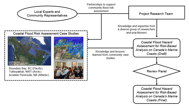
The guideline document was developed through contributor experience and directly from lessons learned from studies in three coastal communities on Canada’s Pacific, Arctic, and Atlantic coasts (Ferguson et al., 2022; Kim et al., 2024 and Rabinovich et al., 2023). Each case study was conducted in partnership with local experts and community representatives to better understand and address local and regional concerns. Partnerships between the core research team, local experts, and community members fostered opportunities for data sharing and collaborative research to enhance the study outcomes and advance knowledge of coastal flood hazards and risk in Canada. The guideline development process is illustrated in Figure 1.2.

1.5 Related Guidance

This document has been written to align with existing applicable Canadian guidelines related to coastal flood hazard assessment. A comprehensive and developing series of guidelines are provided in the Federal Flood Mapping Guidelines Series (FFMGS) including guidelines on lidar acquisition, hydrologic and hydraulic procedures, geomatics, damage estimation, and risk assessment. This document provides guidance on assessing coastal flood hazard to support risk-based analyses on Canada’s marine coasts, expanding upon the description of coastal flood hazard provided in the Federal Hydrologic and Hydraulic Procedures for Flood Hazard Delineation under the FFMGS. Readers are referred to the FFMGS for guidance on damage estimation and risk assessment.

Additional information and guidance specific to the design of buildings and infrastructure can be found in the Coastal Flood Risk Assessment Guidelines for Buildings and Infrastructure Design Applications, published by the National Research Council of Canada (NRC) (Murphy et al., 2020). Murphy et al. (2020) provides guidance specific to hazard and risk assessment of buildings and infrastructure, whereas this guideline more broadly focuses on flood hazard assessment in marine coastal zones in support of risk-based analyses.

Consideration of future sea-level rise is a key aspect for coastal flood hazard assessment to address uncertainties associated with a changing climate. National and regional maps and data files of projected sea-level change across Canada are provided by James et al. (2021).

In addition to federal guidance and international referencing, there are provincial and territorial guidelines available in several jurisdictions and guidance documents from professional practice organizations. This federal guidance is intended to provide assistance for jurisdictions without existing guidance or as an additional reference for communities with existing guidance. It is not intended to supersede local guidance but can be considered alongside any standards of practice or existing guidance.

1.6 Note on Terminology

The concept of risk is often misused. In the context of a hazard assessment, the risk is assessed according to the probability of flooding. Probability of flooding is commonly expressed though return periods or annual exceedance probabilities (AEPs). Section 2.3.4 describes event likelihood in detail. Return periods such as 1-in-100 years can often be misunderstood to mean that an event will happen only once in 100 years. In reality, there is a 1% chance that a 1-in-100-year event will occur in any given year. In this guideline, AEP is used to describe likelihood to provide clarity on the probability of flood hazard.

Coastal flood risk encompasses both the probability of a flood hazard and the consequence of a hazard being realized based on vulnerability, proximity, or exposure (NRCan, 2022). In best practice, risk reduction decision making is based on a range of hazard events with differing likelihoods (as opposed to a single event with a single likelihood) and an understanding of their impacts. More information on risk-based assessments can be found in Murphy et al. (2020). By understanding risk through a range of events, effective risk reduction decisions can be made. Risk is dynamic and changes over time owing to changes in land use, relative sea-level change, and coastal erosion, amongst other factors.

Once a detailed coastal flood hazard assessment is completed, these findings should inform a risk assessment and, subsequently, decisions for current and future priorities related to disaster mitigation and adaptation (see NRCan, 2022).

The following definitions are provided for technical and non-technical terms to clarify their intended definition in this guideline and to prevent misinterpretation. Definitions strive for use of commonly understood language and adequate description for thorough understanding. To support consistency of terminology, the definitions provided below have been gathered from leading sources related to coastal flood assessment, including guidance provided under the FFMGS (NRCan, 2024) and FEMA (n.d.).

Annual Exceedance Probability (AEP): The probability, expressed as a percentage, of a given flood flow or water level occurring or being exceeded in any given year. Flood events are usually expressed in terms of an annual exceedance probability (AEP) or return period. For example, a 1% AEP flood event, and a 100-year flood event, are equivalent. However, the concept of return periods is sometimes misinterpreted by non-technical audiences as a period of time between events (e.g., 100 years until the next 100-year flood) rather than an annual probability. (NRCan, 2023)

Annual Recurrence Interval (ARI): Average Recurrence Interval (ARI) or return period is the expected average period between events of this magnitude or greater if a sufficiently long sample period was used. It is expressed as number of years. This is the generally considered the direct inverse of AEP. The occurrence of a flood event does not reduce the likelihood of a similar or greater flood occurring in the following year or years. Floods with an ARI of n-years could occur 0 to y times within a period of y-years, regardless of if n is greater, equal, or less than y.

Consequence: With respect to flooding, it is the impact, damage, harm, or loss which can be economic, cultural, or environmental that may result from a flood. The impact may be expressed quantitatively (e.g., monetary value, or number of), by category (e.g., high, medium, low), or descriptively.

Event: The realization or instance of a potential flood hazard-generating source (or sources, in the case of compound events) that occurred in the past (historical event) or could occur (hypothetical event). Events are related only to natural processes (sources) and can be characterized by their magnitude or intensity (and associated frequency or probability of occurrence), and spatial or temporal distributions. Indeed, “event-based” flood hazard modelling approaches (e.g., Conner et al., 2011) differ from “response-based” approaches in that the hazard probabilities relate to the hazard source, as opposed to the probability associated with the hazard response (e.g., flood depth in the community). The following are examples of flood hazard events: the 6 December 2010 storm-driven flooding on the Acadian Peninsula, New Brunswick (historical event); a 1% AEP extreme water level event at Belledune, New Brunswick (hypothetical event).

Exposure: The situation of an individual, community, assets, or system located in hazard-prone areas.

Flooding: The temporary inundation by water of normally dry land. (NRCan, 2021)

Flood Mapping: The delineation of a flood on a base map. This typically takes the form of flood lines on a map that show the area that will be covered by water, or the elevation that water would reach, during a specified flood event. The data shown on the maps, may also include flow velocities, depth, other risk parameters, and vulnerabilities. (NRCan, 2021)

Flood Risk: The combination of the probability and negative consequences of a flooding hazard occurring.

Flood Risk Assessment:): Evaluation of hazards and their (negative) consequences in a systematic manner. While some authors use analysis interchangeably with assessment, these guidelines use analysis to describe more focused sub-tasks as part of a broader assessment effort.

Hazard: A potentially damaging physical event, phenomenon or human activity that may cause the loss of life or injury, property damage, social and economic disruption, or environmental degradation

Overland Wave Propagation: “Along low-lying coasts, land that is typically dry may be covered by water during a storm event. Waves advance across the surface of the water in a process called overland wave propagation. As waves move across the land, features, such as high ground, trees, and buildings cause waves to get smaller. If waves cross into open space—like a pond or a golf course—fueled again by strong winds, they may grow larger.” (FEMA, n.d.)

Return Period: – Equivalent to Annual Recurrence Interval (ARI), this is the inverse of AEP, expressed as a number of years. (NRCan, 2022)

Scenario: “Plausible descriptions of how the system and its driving forces may develop […] based on a coherent and internally consistent set of assumptions about key relationships and driving forces.” (Walker et al., 2003)

Storm Surge: The increase (or decrease) in still water level at a coastal site due to meteorological conditions. Storm surge may include wind set-up (or set-down) and barometric set-up (or set-down) (Murphy et al., 2020)

Vulnerability: The conditions determined by physical, social, economic, and environmental factors or processes which increase the susceptibility of an individual, community, valued assets, or systems to the impacts of hazards.” (UNDRR, 2021)

Wave Set-up: “Waves breaking at the coastline push water out and up in front of them, causing an increase in the water level at the coast. This is referred to as the wave set-up. Wave set-up increases the water levels, therefore the combination of wave set-up on top of storm surge is called the total stillwater elevation.” (FEMA, n.d.)

Wave Runup: “In areas with higher ground and steeper shorelines, waves break at the shoreline and water washes up the face of the beach, dune, bluff, or structure that it encounters. This uprush of water is called wave runup.” (FEMA, n.d.)

Wave Overtopping: “Wave overtopping occurs when wave runup reaches the top of the dune or bluff and flows or splashes over into the area behind. Due to these processes, properties located at relatively high elevations above the total stillwater or behind protective structures may be at risk of coastal flooding.” (FEMA, n.d.)

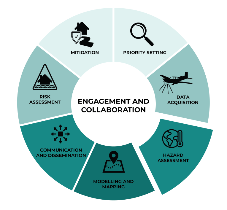
1.7 Framework for Coastal Flood Hazard Assessment for Risk-Based Analysis on Canada’s Marine Coasts

A framework for coastal flood hazard assessment to support risk-based analyses is shown in Figure 1.3. The framework consists of five key components that collectively contribute to robust assessment of coastal flood hazard on Canada’s marine coasts. The framework also illustrates the structure of this guideline document that provides a dedicated chapter for each of the five components. A brief description of each component/chapter is presented below.

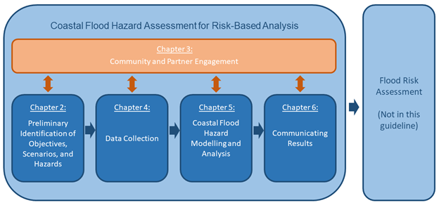
Chapter 2 - Preliminary Identification of Objectives, Scenarios, and Hazards

This chapter is intended to help technical and non-technical individuals understand and scope coastal flood hazard assessments. The chapter summarizes guidance on:

• Establishing objectives, audience, and scope.
• Identifying coastal flood hazards, developing preliminary hazard scenarios, and considering climate change.
• Reviewing background information to build on existing work.
• Establishing project scope to address assessment objectives.

Chapter 3 - Community and Partner Engagement

This chapter offers guidance on fostering meaningful engagement with communities and partners to: establish priorities and scope, build trust, identify opportunities for collaboration, enhance study robustness, and ensure that outcomes provide meaningful contribution to disaster risk management. Community and partner engagement should occur during the entire project and should not be isolated to a particular phase.

Chapter 4 - Data Collection

This chapter provides guidance on identifying and acquiring data commonly needed for coastal flood hazard assessment, including a summary of data resources currently available to practitioners.

Chapter 5 - Coastal Flood Hazard Modelling and Analysis

This chapter summarizes technical guidance for establishing hazard scenarios and modelling coastal flood hazard. Guidance pertaining to storm surge, tsunami, and wave modelling is presented, including considerations to address impacts of sea ice, infrastructure, and climate change.

Chapter 6 - Communicating Results

This chapter summarizes principles of communication, types of communication tools, and communication needs for specific audiences. Key questions to understand assumptions and limitations of modelling are identified for authors to articulate and users to ask. Guidance is provided on communicating hazard assessment findings to support risk-assessment needs and tailoring communication for specific audiences.

Flood Risk Assessment

This component is not part of this guideline but is the next step in identifying who and what are at risk to coastal flooding.

1.8 References

Conner, K. L. C., Kerper, D. R., Winter, L. R., May, C. L. et Schaefer, K. (2012). Coastal flood hazards in San Francisco Bay: A detailed look at variable local flood responses. In Wallendorf, L. A., Jones, C., Ewing, L., Battalio, B. (Eds.), Solutions to Coastal Disasters 2011 (pp. 448-460). American Society of Civil Engineers. https://doi.org/10.1061/41185 (417) 40

Federal Emergency Management Agency (FEMA). (n.d.). An Introduction to FEMA Coastal Floodplain Mapping. https://fema.maps.arcgis.com/apps/MapSeries/index.html?appid=89d2e393f2c64d7cae07264f4d00c19d

Ferguson, S., Provan, M., Murphy, E., & Kim, J. (2022). Numerical Simulation of Coastal Flood Hazard in the Acadian Peninsula Region of New Brunswick (NRC-OCRE-2021-TR-060). National Research Council Canada. https://nrc-publications.canada.ca/eng/view/object/?id=5bb0bbdc-79b0-4870-a9d2-03462932f1c7

James, T. S., Robin, C., Henton, J.A., & Craymer, M. (2021). Relative Sea-level Projections for Canada based on the IPCC Fifth Assessment Report and the NAD83v70VG National Crustal Velocity Model. Natural Resources Canada. https://doi.org/10.4095/327878

Kim, J., Murphy, E., Ferguson, S., Provan, M., & Nistor, I. (2024). Numerical simulation of storm surges in the Beaufort Sea and coastal flood hazards in the Hamlet of Tuktoyaktuk, Northwest Territories (NRC-OCRE-2022-TR-015). National Research Council Canada. https://doi.org/10.4224/40003267

Murphy, E., Lyle, T., Wiebe, J., Hund, S. V., Davies, M., & Williamson, D. (2020). Coastal Flood Risk Assessment Guidelines for Building and Infrastructure Design Applications (CRBCPI-Y5-R2). National Research Council Canada. https://doi.org/10.4224/40002045

Natural Resources Canada. (2021). Federal flood damage estimation guidelines for buildings and infrastructure (version 1.0). Government of Canada. https://doi.org/10.4095/327001

Natural Resources Canada. (2022). Federal land use guide for flood risk areas. Natural Resources Canada. Government of Canada. https://doi.org/10.4095/328955

Natural Resources Canada. (2023). Federal hydrologic and hydraulic procedures for flood hazard delineation (version 2.0). Government of Canada. https://doi.org/10.4095/332156

Natural Resources Canada. (2024). Federal Flood Mapping Guideline Series. https://natural-resources.canada.ca/science-and-data/science-and-research/natural-hazards/flood-mapping/federal-flood-mapping-guidelines-series/25214

Public Safety Canada. (2022). Floods. https://www.publicsafety.gc.ca/cnt/mrgnc-mngmnt/ntrl-hzrds/fld-en.aspx

Rabinovich, A., Thomson, R., and Hastings, N. (2023). Natural hazards in the Boundary Bay region of the Strait of Georgia: A compilation and summary of observations and numerical modeling studies (Canadian Technical Report of Hydrography and Ocean Sciences 366). Fischeries and Oceans Canada.

United Nations. (2016). Report of the open-ended intergovernmental expert working group on indicators and terminology relating to disaster risk reduction. https://www.preventionweb.net/files/50683_oiewgreportenglish.pdf

United Nations Office for Disaster Risk Reduction. (2015). Sendai Framework for Disaster Risk Reduction 2015–2030. United Nations. https://www.undrr.org/quick/11409

United Nations Office for Disaster Risk Reduction. (2021). Disaster risk reduction terminology. https://www.undrr.org/terminology

Walker, W. E., Harremoës, P., Rotmans, J., van der Sluijs, J. P., van Asselt, M. B. A., Janssen, P., & Krayer von Krauss, M. P. (2003). Defining Uncertainty: A Conceptual Basis for Uncertainty Management in Model-Based Decision Support. Integrated Assessment, 4(1), 5–17. https://doi.org/10.1076/iaij.4.1.5.16466

Zevenbergen, C., Cashman, A., Evelpidou, N., Pasche, E., Garvin, S., & Ashley, R. (2010). Urban Flood Management. CRC Press.

2.0 Preliminary Identification of Objectives, Scenarios & Hazards

Lead Authors

Julie Van de Valk (Natural Resources Canada) and Nicky Hastings (Natural Resources Canada)

Contributors

Sean Ferguson (National Research Council Canada) and Enda Murphy (National Research Council Canada)

Suggested Citation

Van de Valk, J. and Hastings, N.L. (2025). Preliminary identification of objectives scenarios, and hazards. In Coastal Flood Hazard Assessment for Risk-Based Analysis on Canada's Marine Coasts. Editors Ferguson, S., Hastings, N.L., Van de Valk, J., Murphy, E., and Kim, J. Government of Canada.

2.1 Introduction

Before a coastal flood hazard project begins, there is a need to clearly understand the objectives and context of the work to be undertaken. This chapter is intended to help individuals with or without a technical background understand and scope coastal flood hazard assessment studies. This chapter is also intended to assist in the preliminary steps of a project, identify the data that need to be collected, and the analyses that need to be conducted to meet community coastal flood hazard assessment needs. While technical experts/engineering firms or in-house specialists often undertake coastal flood hazard project details, this document can also assist community representatives with less technical experience and knowledge to plan out the scoping (objectives, scenarios, hazards) to facilitate a coastal hazard assessment for their community. This chapter is aimed at helping to frame objectives, scenarios, and hazards for decision makers to facilitate a coastal hazard assessment in their community.

2.2 Characterizing Objectives

To meet project objectives, they must first be defined. Project objectives shape many aspects of project scope, and this section discusses common objectives and the implications they have on project scope.

Guiding questions to characterize objectives include the following:

• Who should be involved in characterizing the objectives? Depending on the project, it is likely appropriate that Indigenous Nations, local governments, Rights holders and community members are involved in characterizing the objectives. Community values and preferences can define the vision and overall intent of the project objectives. What are the issues of concern in the community, and how will this affect the thresholds of risk tolerance and mitigation/adaptation in the community?
• Who will use the information generated by the project? Does the audience have a technical background or a non-technical background? What resources do you need to develop to communicate with your audience?
• What will the information be used for? Will it be used for emergency management, engineering design, land use planning, long-term regional planning, community risk assessment, financial risk assessment, or general information? What project outputs are needed for these uses?
• What is the study area? Is the study site-specific, neighbourhood-level, for a watershed or other naturally bounded feature, for Indigenous Territories, for an administrative region, such as a city, province, or nation? For site-specific flood assessments see Murphy et al., (2020).
• What sources contribute to flood hazard? What flood hazards are expected in the area of interest (e.g. tsunami hazards, storm hazards, wave hazards, sea-level rise, or a combination of hazards)? More information is provided on scenario development in Section 2.3.
• What time horizon should be considered? Climate change is a key factor in coastal flooding and the effects vary with time. The lifetime of relevant infrastructure can also dictate what time horizons to consider as can routine municipal planning timelines. The type of questions that are prompting the coastal flood hazard assessment should align with the timelines being assessed in the project.
• What resources and timeline will the project have? The analytical complexity of the project will influence the resources required.
• Will the analysis have to align with any guidelines or funding program requirements? In addition to these federal guidelines, many provinces have guidelines and funding programs with requirements, such as considering the impacts of sea-level rise in analysis.
• What are the roles of the regulator, community staff, and qualified professionals? Can the analysis be done with resources that are an existing part of the lead organization or will external contracts be required?
• What are the output requirements? What is needed in terms of output products? These are further discussed in Chapter 6 and should be characterized in the project scope.

These guiding questions to characterize project objectives and establish a project problem statement lead to scenario development, as discussed in Section 2.3.

2.3 Scenario and Event Development

The concept of a scenario has different meanings to different people and disciplines. For emergency managers, a scenario is a specific, hypothetical event used for emergency planning purposes. For community planners, scenario planning is a decision-making tool to consider potential future development or settlement patterns. In this guideline, a scenario refers to a modelled situation characterized by a set of parameters that represent the natural hazard, as well as the modelled context (such as assumptions about land cover). Scenarios are used to inform planning for future risk reduction by understanding the range of events that can occur and the likelihood of these events occurring. Events are understood as the combination of potential flood hazard-generating sources and are characterized by their extent, magnitude and intensity. Hazard events are not necessarily predictions but help to conceptualize possible future hazard events. Flood hazard events refers to the specific water conditions that are represented in the broader scenario. Background information and community needs and concerns guide the selection of appropriate hazard events to inform the decisions that help prioritize and make smart risk-reduction decisions.

2.3.1 Choosing Hazard Events

The following are aspects to consider in the selection of a hazard event:

• Existing work in the area – Previous studies or work in neighbouring communities may have characterized events with parameters that should be considered for consistency or expansion. This can include a review of academic and government literature as well as policies and actions undertaken by communities and regions including any information on community risk tolerance.
• Project objectives – Different objectives require different modelled events. For example, emergency planning typically looks at low-likelihood and high-consequence events, risk assessment requires a range of events, and engineering design may require a specific event. Guidance on aligning event selection with project objectives is presented in Section 2.3.5.
• Historical events and conditions – Community members may be familiar with historical events, so a selection of these events for analysis or relating these events to events modelled may help with risk communication.
• Timeframe of interest – The timeline for planning and decision making should be used to guide the selection of hazard events.
• Hazard identification and events of concern – Establish priorities comparing the types of hazards and systems at play within the geographic areas of concern. Should any sources of potential hazard be intentionally *excluded* and why (e.g., they are or will be addressed through complementary studies)?
• The number of hazard events – Project budget and resources may influence the number of events that can be feasibly analyzed. Events should be prioritized based on objectives.
• Updating hazard events – As science and knowledge is developed and knowledge is gained from actual events, and climate change models are refined, hazard event characterization should be updated.

Scenarios and events do not all have to be determined before the project starts, but some consideration is important for proper scoping. In outlining a hazard event for a project scope, the following are recommended aspects to communicate. Not all parameters have to be defined in the project scope, but communicating expectations pertaining to the following components will help the project team to establish and accomplish objectives. In the context of a coastal flood hazard assessment, aspects of hazard scenarios should consider:

• Area of interest - Study area
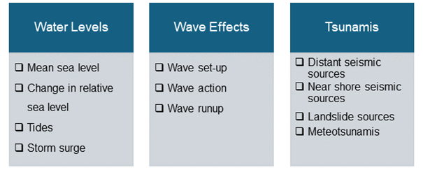
• Hazard sources and components – What sources potentially contribute to the flood hazard? Are storm surge, tides, wave impacts, tsunamis, sea ice, and/or sea-level rise considered? How is the probability of the event calculated? Are the probabilities of contributing sources correlated or independent, and what does this mean for the interpretation of results?
• Connecting coastal areas – Is it necessary to understand or characterize propagation of connecting flood hazards? For example, extending up rivers and estuaries.
• Event Likelihoods - What are the chances or specific likelihoods of a flood event (storm surge, tsunami, etc) that should be addressed?
• Range of Events and Scenarios - What are the range of events and scenarios that should be considered? from the small, relatively likely flood to the large less likely flood event?
• Appropriate Level of Analysis - What resolution of modelling should be used? Coarse? Fine?
• Background Review (see Section 2.4).
• Climate Change -What is the uncertainty? Are changes in storm patterns, ice conditions or intensity considered? Is sea level rise included? And what does this mean for understanding the results?
• Topography - What is represented in the Digital Elevation Model (DEM)? Are structures included in or removed from the topography? What is the required resolution of the topography and bathymetry, and what does this mean for the results?
• Flood Defence - How are flood defences treated? Are dikes removed from the topography or included? Are structures acting as flood defences in the model that aren’t engineered to do so (e.g., a large commercial building diverts flow away from an area that would otherwise be flooded)? And what does this mean for understanding the results? What happens when the capacity of protective works is exceeded? For example, a sea dike that remains intact when significant overtopping occurs versus a dike that is breached.
• Geomorphology - Is the coastline changing? Are there geomorphic hazards alongside flood hazards? – erosion, sedimentation? And what does this mean for understanding the results? How will these considerations be aligned or expressed at the horizon of climate change scenarios?
• Other – Seasonality, river discharges in coastal models? Uplift or subsidence, freeboard? Other changes in the community such as current and future land use and land cover? Post-seismic relaxation and subsidence affecting coastal areas.

Understanding this information will assist the project team in determining appropriate analysis tools or techniques, which, if known, should be described in a project scope.

2.3.2 Identify Study Area

In project scoping, a clear study area should be determined. The study area should include the area of interest and may have to extend to include the following:

• Infrastructure and areas of cultural significance that may be outside of administrative boundaries. Opportunities for inter-community partnerships and efficiencies may exist.
• Modelling of the region is required to derive local coastal parameters. Regional models may exist in some areas from other projects, but if they do not, a regional model may need to be developed to establish parameters for a higher-resolution local model. Regional models are typically lower resolution than the primary study area of interest.
• Distant hazard sources for tsunamis, such as landslides or earthquakes, may be far from communities. Tsunami sources and impact areas need to be included in the modelling area at some resolution. If hazard sources are outside of the study area of interest, nested modelling approaches with large models at lower resolution may be used.
• Calibration/validation locations that may be outside the main study area.

2.3.3 Identify Hazard Sources and Components

Coastal flood hazards have a variety of sources and interact with a variety of systems. Hazard sources can be single sources or multiple sources that are coupled or compounded. Most hazards will be altered due to climate change, and climate change should be considered in any analysis. Figure 2.1 shows coastal flood hazard sources.

These sources may act alone, or in combination, to generate coastal floods. Events that are comprised of multiple hazard sources will have a probability of occurrence representative of the combined probabilities of the individual hazard sources. Identifying hazard sources (and possible combinations thereof) for analysis is a key aspect of detailed event development as described in Chapter 5. However, for preliminary identification, hazards of interest that impact the study area should be identified in the project scope.

Climate change affects many of these hazard sources. There is a fairly clear understanding of the effect of climate change on sea-level rise for given shared socio-economic pathways or emissions scenarios, although there remains uncertainty in future timing of sea level changes. There is more uncertainty in the link between climate change and changes in storminess (Greenan et al., 2018). The magnitude of sea-level change due to climate change depends on the location, the planning horizon, and the global emissions scenario. These can be defined in the project scope or considered through future work on detailed event definition.

Hazard sources (such as those described above) represent the natural system characteristics and driving processes that contribute to hazardous conditions. Hazard pathways represent the linkage between hazardous conditions and a vulnerable receptor (e.g. a coastal community). As described by Murphy et al. (2020), pathways include direct inundation, erosion, barrier overtopping, and barrier bypassing.

2.3.4 Likelihood of an Event

Each event has an associated likelihood. Event likelihood is typically derived from a combined likelihood of multiple hazard components and is typically represented as a return period or annual exceedance probability (AEP). A range of likelihoods are required for risk assessment and are recommended for emergency planning purposes. Many jurisdictions also have a designated flood for design and land use planning. However, most modern guidance recommends a risk-based approach, where different likelihood events are used for different land uses depending on the consequences of inundation.

• Events with AEP exceeding 10% are typically considered high probability and sometimes referred to as nuisance flooding.
• 10% to 2% AEP events are typically considered medium probability events.
• 2% to 1% AEP events are considered medium to low probability events.
• 1% to 0.2% AEP events are used widely across Canada as designated flood levels.
• 0.1% (or lower) AEP events are considered low probability events on an annual basis, and are rarely used to guide flood risk management in Canada, but are considered for other natural hazards (e.g. tsunami, or earthquake) and in other jurisdictions around the world.

The probability of events can be difficult to communicate in a way that people can relate to. Two common ways of stating event probabilities are given in the first two columns of Table 2.1 and more generally in Figure 2.3. In Table 2.1, the chances of these events occurring over a given time span are given as an additional communication strategy.

Return Period Footnote 1 (years)	Annual Exceedance Probability Footnote 2 (%)	Chance of Exceedance over 25 Years Footnote 3 (%)	Chance of Exceedance over 50 Years Footnote 3 (%)
1-in-5	20	100 Footnote 4	100 Footnote 4
1-in-10	10	93	99
1-in-20	5	72	92
1-in-50	2	40	64
1-in-100	1	22	39
1-in-200	0.5	12	22
1-in-500	0.2	5	10
1-in-1000	0.1	2	5

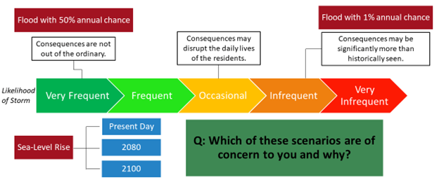
For tsunami modelling, worst case scenarios should be explored, whereas for storm hazard modelling, higher-likelihood scenarios will likely be of more interest and usefulness. Tsunami likelihood often has significant uncertainty.

2.3.5 Number of Events and Scenarios

When hazard sources, event likelihoods, potential pathways to flooding (e.g. dyke breaches, direct inundation), risk management scenarios, future climate scenarios, and other factors are combined, there can be an almost infinite number of scenarios. A risk assessment may consider several storm surge event likelihoods under different sea level-rise projections to understand potential, future annualized damages. For example, for both the Atlantic and Arctic case studies, six storm surge events with unique AEPs were evaluated under present-day sea level conditions as well as three relative sea-level rise scenarios. Murphy et al. (2020) and NRCan (2021) describe the importance of multi-event/scenario approaches that consider a range of likelihoods and potential damage outcomes to adequately quantify risk. The number of events and scenarios required will vary based on the purpose of the risk assessment (e.g. preliminary, or detailed), the number and types of hazards in the area, potential tipping points in consequences (e.g. overtopping of a dyke), the number of risk management strategies or measures being considered, timeframes for risk management planning, and a host of other factors. The selection of event AEPs has the potential to impact results; for example, Ward et al. (2011) found the use of only three AEPs resulted in an overestimation of annual risk between 33% and 100%.

2.3.6 Determining Appropriate Detail for Analysis

A variety of analytical methods can be used to support hazard modelling and other technical tasks, with varying levels of detail. The level of analytical detail required will depend on the purpose of the hazard and/or risk assessment, and methods should be selected accordingly. For risk assessments covering a broad geographic area, perhaps low analytical detail is acceptable in order to balance computational demand with the need for broad results. For risk assessments of small areas or specific properties and infrastructure, a much higher level of detail is required. More detailed modelling requires more effort be put toward input data, a higher model resolution, and more sophisticated and computationally intensive modelling, amongst other things. Accurately describing the level of detail required in analysis is a key part of scoping projects as it helps ensure that potential project bids provide comparable products. The following list summarizes some modelling considerations that affect level of detail:

• Model complexity. Simplified modelling techniques (e.g. bathtub modelling – see Section 5.4.4) may be suitable to support rough approximation of flood hazard based on water elevation alone. However, more-complex modelling techniques (e.g. two-dimensional hydrodynamic modelling) may provide a more-realistic representation of flood hazard, as well as additional information pertaining to flow velocity, flood propagation, and flood duration. Modelling complexity will influence data requirements, analytical effort, and computational demand.
• Wave modelling versus wave estimation. If waves are a significant hazard in the study area, the analysis of wave impacts will be more important. For some areas, waves are relatively minor hazards, in which case generalized estimates of wave effects are adequate. In other areas, wave hazard is significant, and localized dynamic modelling of waves is required. High-quality wave modelling includes analysis of local wind direction, collection of localized shoreline profiles or a gridded bathymetric digital elevation model (DEM), and specific hydrodynamic modelling.
• Model resolution. Spatial resolution (as well as temporal resolution for hydrodynamic models) will affect modelling detail and computational demand. Both spatial and temporal resolution are somewhat limited by the resolution and accuracy of the underlying data. For example, to avoid interpolation inaccuracies, high-resolution topography data must be available to support modelling with high-spatial-resolution. The model resolution required (spatial and temporal) depends on the objectives of the hazard and/or risk assessment.
• Horizontal and vertical accuracy. Clear expectations and limitations around horizontal and vertical accuracy should be discussed in project planning. Calibration and validation will demonstrate the model accuracy, and this must align with intended model use.

2.4 Background Review

It is important to review available data in the development of a project scope, as there may be some key information that must be either collected before a hazard assessment or incorporated into the project. Identifying relevant and available information is essential in scoping an implementable project. Providing this information in the project scope ensures that an accurate and reasonable project plan can be developed.

2.4.1 Identification of Partners, Stakeholders, and Rightsholders

At the earliest stages in the project, partners, community stakeholders, and Indigenous rightsholders should be a part of the project planning process. They can provide essential input for the characterization of objectives, scenario development, and information sources. Chapter 3 has more information about community and partner engagement, including guidance on how to identify and engage with communities and partners.

2.4.2 Previous Studies and Flood Risk Management Initiatives

Many coastal communities have examined coastal flood hazards through previous studies. To work efficiently and build on existing understanding, previous studies and flood risk management initiatives should be identified early in the project planning process. Information sources can include academic journal articles, consulting reports, and reports or studies from multiple levels of government. A comprehensive review should be completed before project completion and relevant materials listed in project scopes. Connecting with local researchers, practitioners, government representatives, and community organizations may be helpful in ensuring all relevant information is found, as some may not be searchable on online databases. Previous studies and flood risk management initiatives relevant to coastal flood hazard could include:

• Coastal geomorphology assessments.
• Tidal or storm surge frequency analyses.
• Previous, regional, or neighbouring coastal flood hazard assessments.
• Previous, regional, or neighbouring tsunami studies.
• Biology or ecosystem assessments in the area.
• Environmental Impact Assessments.
• Riverine hazard assessments.
• Studies that informed design of coastal infrastructure.
• Details of past flood risk management projects, such as beach nourishment, harbour dredging, and coastal diking.

2.4.3 Past Flood Events

Information about past flood events is essential in calibrating and validating coastal flood hazard models. There are many long-term benefits of having an established program for post-flood data collection. Past flood events that reflect aspects of the hazard scenarios identified in the scenario development phase should be identified. Past flood events can be identified from previous studies, community historical records, photos, water level or weather records, Indigenous knowledge, sedimentary records, other physical indicators of floods or high-water levels, and spatial data representing past floods.^{Footnote 1} More detail about these data sources is included in Chapter 4 for detailed collection once projects are underway. For scoping projects, it is important to have an understanding of available data about past flood events—if no information is readily available, additional effort will have to be spent to gather information for calibration and validation.

2.4.4 Model Input Data

Available model input data must be identified and reviewed as part of project scoping to ensure an accurate scope that allows for additional data collection, if required. More information about data collection is provided in Chapter 4. The list below summarizes input data commonly required for coastal flood hazard modelling as well as key considerations pertaining to each data type. The list can be used to support scope development and identification of data gaps but should be viewed as preliminary and non-exhaustive. Specialist advice and input should be sought to identify data needs and gaps, and to ensure available datasets are adequate to support risk assessment. Data gaps or shortcomings are often only uncovered following thorough review, analysis, and quality checks. Therefore, it may be prudent to put budget and schedule contingencies in place at the beginning of a risk assessment, to support data acquisition, if needed.

The data required for modelling depends on the project objectives and the scenarios identified as described in Sections 2.2 and 2.3.

Elevation Data: Topography and bathymetry are required for all coastal flood hazard modelling. The resolution of the data must align with the desired model resolution. The extent of the data must include the entire model extent, including on-shore areas where inundation or runup are possible, and offshore hazard start-zone areas. Nearshore and tidal zone elevation information is especially important if wave runup analysis is planned. The Federal Flood Mapping Guidelines Series provide some information about collection of lidar data and development of a digital elevation model (DEM). As coastal regions are dynamic, elevation data must be relatively recent to accurately represent current-day conditions. If no topographic or bathymetric information exists of a suitable quality and recency, it will have to be collected before a flood hazard assessment begins. This can add significant expense and time onto a project and should be confirmed before scoping a flood hazard project. Information about geomorphological changes along the coastline is also relevant to analysis and should be identified where available. There is often also value to obtaining historical elevation data to support calibration and validation. The calibration /validation process should be undertaken using topographic/bathymetric data that is physically concurrent with the conditions under which the calibration (or validation) event occurred. For example, if coastal erosion or accretion has significantly altered the foreshore since the calibration event occurred, a process that calibrates the present-day model to historical water levels would make the model “right for the wrong reasons.”

Tidal Information: Information about tidal levels is an important input as an initializing water level in modelling. This is typically readily available from local tidal charts.

Storm-Related Water Level Information: If the scenarios of interest include analysis of storm impacts, water level gauge and meteorological records could be required. In scoping the study, information about tidal and meteorological stations should be identified including: station location, duration of record, and parameters recorded. For high-quality analysis, highly localized information is required. If local information throughout the study area is not available, additional effort may be required in the project scope to collect or simulate the information. The duration of record is also important, especially to estimate low-likelihood events. If low-likelihood events are of interest but records are relatively short, additional effort may be required in the project scope to synthesize extended records. More detail about storm-related water level data collection is provided in Chapter 4.

Tsunami Source Information: If tsunami hazards are a part of the analysis, source models are required. Source models can include seismic sources, aerial and submarine landslide sources, and meteorological forcing. Identifying source information to match the scenarios selected is a key factor in determining project scope—if sources are not available in the region, additional effort will be required to develop source models. If sources are available that align with the scenarios, less effort is required for the project.

Relative Sea-Level Change: Simply put, relative sea-level rise is determined by changes in mean sea levels and land elevation. Changes in mean sea level due to sea-level rise vary along Canadian coasts. In areas with high seismic influence, the effects of land uplift or subsidence following significant earthquakes can affect future sea level projections. At this time, however, guidance cannot be provided as to how to incorporate these effects. Relative sea-level rise projections are accessible through an NRCan resource—Relative Sea-Level Projections for Canada based on the IPCC Fifth Assessment Report and the NAD83v70VG National Crustal Velocity Model (James et al., 2021). These are provided for a variety of time horizons, potential climate scenarios, and incorporate regional differences in rates of change in land elevation. These projections have now been revised to incorporate new global sea-level projections from the IPCC Sixth Assessment Report.

Sea-ice extents and thickness are important information in areas that experience winter freezes along the coastlines. This information is typically available through regional monitoring. Land use and land cover information is important to characterize surface roughness for hydrodynamic modelling. This information is usually available from regional spatial datasets. Built structures in the area are important for detailed modelling, as they impact waves and water levels, and can often be found from local or open-source building inventories. Where rivers meet coastlines, there can also be additional flooding from discharge volumes or overland flooding from riverine sources along coastlines. Data pertaining to riverine flood hazards can be available from river flood hazard studies and should be incorporated where relevant.

2.4.5 Community Context and Background Review

General information about community context should be explored in the preliminary phases of a project. General knowledge about a community that is relevant to articulating the scope of a study includes historical patterns of human settlement, demographics, physical characteristics of the built environment, and administrative jurisdictions. When scenarios include future time horizons, such as 2050 or 2100, the community context (e.g., development location and density, population location and density, infrastructure, dike crest elevations) is also likely to change over the same time period. For risk assessment, if predictions for community change are available, they can be incorporated and may change the study area (e.g., potential community retreat or relocation sites may be of interest for inclusion in the model study area).

2.5 Establishing Project Scope

The project scope can be established based on the objectives, hazard scenarios, and available information, and should articulate a clear plan for achieving project objectives. This scope, including all components discussed above, can be used for project planning including requests for proposals, developing work plans, accurate cost estimation, and selection of a suitably qualified professional. To summarize the sections above, clear, specific information should be provided on the following aspects:

• Project introduction
• Project objectives
• Analysis parameters
  • Spatial extent of study area
  • Required resolution
  • Methodology requirements
• Scenarios for analysis
  • Hazard sources for analysis
  • Number of scenarios
  • Desired likelihood of scenarios
  • Consideration of climate change
• Available background information
  • Project partners, stakeholders, and rightsholders
  • Previous or relevant studies
  • Past flood event information
  • Available model input data
  • Community context information
• Community engagement expectations (see Chapter 3)
• Required outputs
  • Mapped results
  • Data outputs
  • Model set-up files
  • Technical project documentation
  • Project communication materials

Other information often provided in a project scope includes timeline, cost limitations, administrative and contracting requirements, submission requirements, and other considerations as dictated by procurement policy.

2.6 References

Greenan, B. J. W., James, T. S., Loder, J. W., Pepin, P., Azetsu-Scott, K., Ianson, D., Hamme, R. C., Gilbert, D., Tremblay, J.-E., Wang, X. L., & Perrie, W. (2019). Changes in oceans surrounding Canada. In Bush, E., Lemmen, D.S. (Eds.) Canada’s Changing Climate Report (pp. 343–423). Government of Canada. https://changingclimate.ca/CCCR2019/

James, T. S., Robin, C., Henton, J. A., & Craymer, M. (2021). Relative Sea-level Projections for Canada based on the IPCC Fifth Assessment Report and the NAD83v70VG National Crustal Velocity Model. Natural Resources Canada. https://doi.org/10.4095/327878

Murphy, E., Lyle, T., Wiebe, J., Hund, S. V., Davies, M., & Williamson, D. (2020). Coastal Flood Risk Assessment Guidelines for Building and Infrastructure Design Applications (CRBCPI-Y5-R2). National Research Council Canada.

Ward, P. J., de Moel, H., & Aerts, J. C. J. H. (2011). How are flood risk estimates affected by the choice of return-periods? Natural Hazards and Earth System Sciences, 11(12), 3181–3195. http:/doi.org/10.5194/nhess-11-3181-2011.

3.0 Community and Partner Engagement

Lead Authors

Nicky Hastings (Natural Resources Canada) and Julie Van de Valk (Natural Resources Canada)

Contributors

Mike Ellerbeck (Natural Resources Canada), Zheng Ki Yip (Natural Resources Canada), and Brent Baron (Indigenous Services Canada)

Suggested Citation

Hastings, N.L. and Van de Valk, J. (2025). Community and Partner Engagement. In Coastal Flood Hazard Assessment for Risk-Based Analysis on Canada's Marine Coasts. Editors Ferguson, S., Hastings, N.L., Van de Valk, J., Murphy, E., and Kim, J. Government of Canada.

3.1 Introduction

Community engagement is a vital part of any project, as communities have a unique relationship and understanding of an area. Those with the closest ties to a coastline will be the most impacted by any flooding or flood risk–reduction projects. Typically, those with the closest ties to a coastline will be local communities, Indigenous Nations and rightsholders, and other stakeholders. Community members may have been present during historic flood events and will have a strong connection to the region. In particular, the perspectives of local Indigenous communities are essential to provide a holistic and broader view of the region. Community, partner, and rightsholder engagement throughout a coastal flood hazard assessment is helpful in ensuring that studies meet community needs and that community understanding of flood hazards is increased. Depending on the project, engagement can be targeted to the public or a narrower group of stakeholders and rightsholders. This section will explore the principles of engagement and who to include.

3.2 What to Know Before Engaging

Before engaging with communities, stakeholders, or rightsholders, it is important to gather information about the community context. The following list summarizes key items that should be considered prior to engaging with communities and partners:

• What is the project's duration and how many participants will be involved? Are there any timing constraints that may impact the project?
• What is the project’s objective? Will it develop objective technical information for further use, or is it part of a larger project that will make decisions for local communities on land use and flood defences?
• Have there been any recent major or nuisance coastal flood events in the community?
• Are there past/ongoing studies related to coastal flooding in the region and, if so, who was/is involved?
• Are there any sensitive political issues within or between communities that may be affected by project activities or outcomes?
• What are the potential impacts of the work on the community?
• Are there other major projects happening in the area?
• Has there been any media coverage about the community or topics related to the proposed project work?
• Has there been any indication of concern in the community over the proposed project or related issues?

The following list summarizes additional items that should be understood prior to engaging with Indigenous communities:

• Are there Treaties, Treaty Negotiations, Assertions, Land Use Plans, or other documents that may have engagement requirements?
• What are the governance structures for the community? Is governance based on a council structure, hereditary leadership, Nation associations, etc.?
• Is there potential for adverse impact on Section 35 Aboriginal and Treaty Rights (i.e., adverse impacts on traditional activities in the community: hunting, fishing, ceremonial, etc.)?
• What are the past and ongoing colonial impacts in the area? Is there a history of resettlement, contention over land usage and ownership, industrial or infrastructure projects in the area that may be relevant to the coastal flood hazard project?
• What Indigenous names are used for an area, and what can be done to respect Indigenous place names?
• Are Indigenous reserve lands protected by flood defences on Indigenous or non-Indigenous lands, and if so, what is the associated history and current First Nation perspective?

3.3 Principles of Partnership and Community Engagement

The following are four key principles for partnership and community engagement:

• Build awareness and understanding of the community – Consider the community culture, economic conditions, social networks, political structures, norms and values, demographic trends, history, hazards and risks, and previous experience with engagement. A literature and news review provides an excellent first step to understanding the community.
• Go to the community – Establish relationships, build trust, work with the formal and informal leadership, seek commitment from community organizations and leaders to create processes for mobilizing the community.
• Partnership – Build a trusted relationship; communicate and collaborate regularly and often to keep all partners aware of priorities within the respective institutions. Partnership documentation, such as agreements, can help sustain the research when the community organization staff changes.
• Communication – Tailor communication to the target audience. Technical and scientific concepts/information may need to be simplified to facilitate communication with non-technical audiences.

In addition to the above-listed principles, the following list summarizes recommended principles specific to engagement with Indigenous communities:

• Historical exploitation – Recognize the potential for a history of exploitation in the community and possibly a distrust of researchers and scientists. Listen to community feedback on the project. Use a variety of participation strategies. Allow extra time for building relationships and trust. Include local customs in interventions. Demonstrate respect and inclusion to the fullest extent possible.
• Allow adequate time for engagement – Many Indigenous communities are inundated with requests to engage and may be dealing with more pressing community issues.
• Consider an interconnected perspective – Indigenous Peoples may hold the perspective where the land is a living being, and everything is related and interconnected. Plants and animals may be considered as teachers and sources of information about the land and changes related to flooding, such as climate change.
• Storytelling – Many communities use storytelling as a powerful knowledge-sharing tool to understand and transfer knowledge about the land. Any Oral or Traditional Knowledge shared should be shared only with the express permission and acknowledgement of the storyteller.
• Consultation – It is essential to consult with elders, young people, hunters and trappers associations, community corporations, hereditary leaders, and elected officials.

Refer to Section 6.2 for principles of communication.

3.4 Who to Include and How

Robust coastal flood hazard assessment often requires a multi-disciplinary approach involving collaboration amongst practitioners, subject-matter experts, and other representatives. All voices are important and should be heard, but not every voice will have equal weight in the process. For example, input from First Nations should usually be given far more weight in discussions and decisions than input from a small special interest group with a more peripheral interest in the project.

Ocean and coastal jurisdictions are managed by a wide range of governmental jurisdictions. West Coast Environmental Law has developed an infographic depicting the jurisdictions responsible for each zone of a coastal area in BC. This can be a helpful as a guidance to understand what government partners may play a role in the assessment (WCEL, 2018).

The following list summarizes general groups that may contribute to coastal flood hazard assessment:

• Partners – Partners are those who are involved in the work. Partners should include those generating scientific and Traditional Knowledge and the decision makers, who will use the findings to inform mitigation and adaptation strategies, and public awareness. These can include a range of partners from academics, consultants, community staff, and non-profit organizations. Clearly define who is the creator of data, consumer of data, compiler of data, and project funder.
  • Data-sharing agreements can be set up with partners to help establish formal arrangements that detail what data is shared and its appropriate use.
  • Comprehensive project plans and charters endorsed by team members help define project objectives, budget, scope, expectations, outcomes, timelines, and associated risks.
• Steering committee/advisory group – Depending on the scope and scale of the assessment, it may be necessary to establish a steering committee or advisory group. Advisory groups bring context and value to the project and become familiar with the content through participation on the committee. There are various types of advisory groups, including technical advisory groups and general advisory groups. A term of reference can be written to establish roles, responsibilities, and governance. An advisory group shares project knowledge and allows committee members to contribute to, understand, and use the project results once it is complete. The committee/advisory group can be either an existing group or a new group. In developing this group, think clearly about those who are generators of knowledge (scientific and Traditional) and decision makers.
• Community representatives – This is a potentially broad group of individuals, including the public, who are interested in the work and can be affected by, or can affect, the hazard. These could include residents living in an area of coastal flooding, neighbouring communities, or infrastructure owners and operators in the region. Local knowledge from community representatives can often be used to supplement data resources and improve technical analyses (see Section 4.3).
• Title and Rightsholders - Indigenous Nations with connection to the land should be considered as rightsholders in projects and direction for the project should be sought from them.
  • Be prepared to cover for honorariums when consulting with stakeholders. Many of these groups can provide invaluable knowledge about the region and should be compensated for sharing this knowledge. For instance, this is important when engaging with community elders.
  • Referencing Indigenous knowledge should be done with guidance on how and what Traditional Knowledge can be published.
  • The organization you work for can impact the type of engagement with a community, given the history of past engagement and historic colonial practices.

3.5 Governance for Successful Engagement

• The duty to consult Indigenous communities – Article 19 of the United Nations Declaration on the Rights of Indigenous Peoples (United Nations, 2007) states: "States shall consult and cooperate in good faith with indigenous peoples concerned through their representative institutions to obtain their free, prior and informed consent before adopting and implementing legislative or administrative measures that may affect them."
• Accountability – Clearly identify a person responsible for community outreach, to ensure that communication and outreach takes place and is part of the project work.
• Role clarity – Are the roles and responsibilities of each of the parties laid out? A project charter for project partners or a term of reference for committee members can be helpful in clearly defining roles and expectations.
• Authority – All input that is collected should have a predetermined mechanism for being addressed or included in the project. A central point of contact for the project should be established who ensures that feedback is responded to.
• Transparency – Project results should be open, transparent, and communicated as widely as possible in a timely manner.
• Commitment – To ensure success, project partners and committee members must be able to commit to the time required for the success of the project. Scoping the time required through a project charter or committee terms of reference is key to ensuring this.

3.6 Engagement Plan

For a lengthy project, having an engagement plan can help to ensure the success and uptake of the project. Engaging with stakeholders takes time and resources and should be factored into the overall project plan. A stakeholder engagement plan should be developed in partnership with project stakeholders and include the following items:

• Clearly defined touchpoints between project team members and community representatives in the form of meetings, online feedback, one-on-one conversations, surveys, or other options.
• Dates and durations for touchpoints that are outlined far in advance and in alignment with the community's schedule.
• Specific goals for touchpoints that are defined through consideration of the needs of project partners and project workplans.
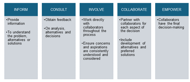
• Spectrum of public participation goals (Figure 3.1).

Chapter 5 of the National Research Council Canada’s Nature-based infrastructure for coastal flood and erosion risk management: a Canadian design guide (Murphy et al., 2024) can be consulted to provide additional resources on Key Principles for Effective Engagement. The guide provides a section that highlights a range of Tools and Resources such as shoreline walks, photovoice, surveys, community dinners, physical modes, etc. which would enhance the engagement process.

3.7 Transition at Project Conclusion

In the final stretch of the project, there are some important decisions to be made to transition and enable the work generated to support future flood risk modelling and decision making.

• Ownership of intellectual property – Once the project is complete, there is potential for publication of results, as well as data and model storage. Plans for this should be made as early in the project as possible to ensure transparency with community representatives and the arrangement of permissions to share intellectual property as required. As dictated by OCAP principles, Indigenous communities should be in control of how data and information about their populations is shared.
• Training and knowledge transfer – Training and knowledge transfer requires the project team to empower the community to use the information developed in the project to meet their needs. This is a key part of community engagement. Each community will have different capabilities and needs, and they can include:
  • Rerunning the model with different parameters or additional scenarios.
  • Building on the model through future projects.
  • Using the model results for community planning.
  • Using the model results for risk assessment and risk-reduction decision making.
• Documentation for repeatability – New coastal flood hazard models will need to be generated over time as conditions change. For example, alteration of the coastal zone may affect how floodwaters and waves interact with the land. When only a report is left with the community, model results cannot be rerun with new conditions or built upon in future projects. Models should be documented and shared with project partners. Ensuring that models are documented and shared with project funders and partners as outlined in Chapter 6 will help ensure they can be built on in the future.

3.8 References

First Nations Information Governance Centre. (2021). The First Nations Principles of OCAP^®. https://fnigc.ca/ocap-training/

International association of public participation. (2024). Advancing the practice of public participation. https://www.iap2.org/page/pillars#

United Nations. (2007). United Nations Declaration on the Rights of Indigenous Peoples.

West Coast Environmental Law (WCEL). (2018). Jurisdiction in coastal BC. https://www.wcel.org/sites/default/files/publications/2018-05-coastaljurisdiction-infographic-updated.pdf

Murphy, E., Cornett, A., Van Proodij, D., Mulligan, R.P. (2024). Nature-based infrastructure for coastal flood and erosion risk management: a Canadian design guide. National Research Council. 348p. https://doi.org/10.4224/40003325

4.0 Data Collection

Lead Authors

Sean Ferguson (National Research Council Canada), Nicky Hastings (Natural Resources Canada), Joseph Kim (University of Ottawa), Enda Murphy (National Research Council Canada), Charles Papasodoro (Natural Resources Canada), Lucinda Leonard (University of Victoria), Blair Greenan (Fisheries and Oceans Canada), Thomas James (Natural Resources Canada), Kelin Wang (Natural Resources Canada), Gwyn Lintern (Natural Resources Canada), and Mark Rankin (Ocean Networks Canada)

Contributors

Fatima Nemati (University of Victoria), David Bélanger (Natural Resources Canada), and Guillaume Légaré-Couture (Natural Resources Canada)

Suggested Citation

Ferguson, S., Hastings, N.L., Kim, J., Murphy, E., Papasodoro, C., Leonard, L., Greenan, B., James, T., Wang, K., Lintern. G., and Rankin, M. (2025). Data Collection. In Coastal Flood Hazard Assessment for Risk-Based Analysis on Canada's Marine Coasts. Editors Ferguson, S., Hastings, N.L., Van de Valk, J., Murphy, E., and Kim, J. Government of Canada.

4.1 Introduction

Data collection is a crucial component of the coastal flood hazard assessment process. This chapter provides guidance on identifying and acquiring data commonly needed for coastal flood hazard modelling and analysis, including a summary of data resources currently available to practitioners.

4.2 Elevation Data: Bathymetry and Topography

Elevation data are a key component of numerical hydrodynamic model development and simulation of storm surge. The quality of the bathymetric data (i.e., resolution, accuracy, and age/relevance) is crucial to the generation and evolution of the simulated storm surge within the model domain. Similarly, high-quality topographic data are essential to support accurate estimation of overland inundation and flood propagation.

The resolution and accuracy of bathymetric data required for storm surge modelling depend on the purpose of the model. For example, coarse regional- or global-scale bathymetric datasets, or data extracted from navigational charts, may be sufficient for regional-scale storm surge modelling, focused on simulating elevated water levels over a broad geographic range in low detail. However, high-resolution bathymetric data may need to be acquired to support detailed storm surge simulation at the coast, community-scale hazard assessment, and simulation of overland inundation. Likewise, high-resolution data may be necessary to support modelling in nearshore regions close to the area of interest, whereas coarse-resolution datasets may be suitable for modelling deepwater regions.

The resolution and accuracy of topographic data required depends on the subsequent risk assessment and damage estimation needs. Practitioners should consider the spatial scale of the assets in the community (or communities) of interest for which they intend to provide hazard information. For example, if flow around buildings and other obstacles must be captured in the model, then topographic data must be acquired at a resolution to support this type of analysis.

4.2.1 Data

A number of bathymetric and topographic data resources may be available to support hazard assessment. The Federal Geomatics Guidelines for Flood Mapping provide guidance on topographic elevation data for flood mapping. In addition, the current section provides a summary of potential elevation sources more specific to coastal flood hazards. Depending on the geographic location and scope of the hazard assessment, practitioners may need to explore other bathymetric and topographic datasets to support their analyses. Practitioners should be aware that data sharing agreements may be needed that may outline limitations of use.

The Canadian Hydrographic Service (CHS) provides publicly available bathymetric data intended for non-navigational (NONNA) use that can be downloaded via an online portal (CHS, 2018). More precisely, the NONNA-10 product is a multi-source bathymetric dataset leveraging all data managed by the CHS, including single-beam/multibeam echosounder and airborne bathymetric lidar datasets. The spatial resolution of the NONNA-10 product varies depending on latitude as follows (CHS, 2018):

• South of 68°N the products = 0.1° latitude X 0.1° longitude (0.0001 degrees)
• 68°N-80°N the products = 0.1° latitude X 0.2° longitude (0.0002 degrees)
• 80°N and north the products = 0.1° latitude X 0.4° longitude (0.0004 degrees)

Practitioners are encouraged to enquire with CHS for guidance on availability, vertical datum, acquisition, and pricing of best-available bathymetry products for specific locations.

The General Bathymetric Chart of the Oceans (GEBCO) organization provides publicly available bathymetric data covering the world’s oceans (GEBCO, 2020a). The most recent bathymetric products released by GEBCO in 2019 and 2020 provide global coverage over a 15 arc-second grid (GEBCO, 2020b, 2020c).

It is often challenging to find bathymetry datasets in nearshore regions with shallow water owing to technical and practical limitations of data sensing and acquisition equipment; nearshore waters may be prohibitively shallow to support boat-based bathymetric surveying. However, technologies such as airborne topo-bathymetric lidar aim to address this gap, enabling bathymetric surveying in shallow water. For more details on airborne topo-bathymetric lidar, see Appendix 5 from the Federal Airborne Lidar Data Acquisition Guideline, version 3.0 (NRCan, 2020).

Practitioners should be conscious of the utility, limitations, and level of processing associated with topographic lidar-derived datasets. For example, digital terrain models (DTMs) provide a bare-earth representation of the earth’s surface (i.e., free of vegetation, buildings, and other structures), whereas digital surface models (DSMs) represent the elevation of the bare-earth surface plus any surficial coverings (Zhou, 2017). The High-Resolution Digital Elevation Model (HRDEM), which is openly available on Canada’s Open Government portal, provides open access to currently available high-resolution elevation data across Canada and includes both DTMs and DSMs (NRCan, 2019a). The HRDEM product integrates lidar data acquired by multiple partners across the country, and the coverage will keep evolving based on the availability of new lidar data. If areas of interest are not covered yet by the HRDEM product, practitioners are encouraged to enquire about topographic data availability from provincial/territorial governments, municipal governments, and local research institutions, particularly if specialty products (e.g., hydro-enforced elevation products or lidar point data) are required.

4.2.2 Datums

Applying an appropriate and common spatial reference system is crucial to the integrity of any project involving geospatial data integration, including coastal flood hazard assessment. Topographic elevation datasets are usually referenced to geoid-or leveling-based height systems (e.g., CGVD2013 or CGVD28 in Canada), whereas coastal bathymetric datasets are typically referenced to chart datum (e.g., lower low water large tide, LLWLT). The fundamental differences between vertical land and ocean datums reinforce the need for appropriate and accurate conversion.

The Federal Geomatics Guidelines for Flood Mapping (NRCan, 2019b) provide recommendations for vertical and horizontal reference systems of geospatial datasets used in flood mapping. They are based on the most current datum and geoid model defined by NRCan. The same reference systems are recommended for coastal flood hazard assessment.

NRCan offers a variety of tools to convert between orthometric reference systems, ellipsoid reference systems, and epochs (Government of Canada, 2021a). Amongst these tools, the GPS·H software is a convenient tool that allows such vertical transformation on point coordinates (Government of Canada, 2021b). NRCan also provides multiple geoid grids to perform transformations on rasters. Those grids include the CGG2013a geoid model defining CGVD2013, the HTv2.0 hybrid geoid models for epochs 1997, 2002, and 2010; and grids to convert between CGVD28 and CGVD2013 for the same three epochs. Those grids can be downloaded, resampled/meshed to the appropriate pixel spacing (e.g., using tools such as gdal_warp) and then used for the transformations. NRCan’s geodetic tools and reference system information are accessible here: (https://www.nrcan.gc.ca/maps-tools-and-publications/geodetic-reference-systems/18766)

For conversions from chart datum to ellipsoid or orthometric reference systems, users are encouraged to use the Canadian Continuous Vertical Datum for Canadian Waters (Robin et al., 2016) process developed by CHS and NRCan and the applicable Hydrographic Vertical Separation Surfaces (HyVSEP/SEP) for the survey area. HyVSEP/SEP are available for all tidal waters in Canada and can be obtained by request to CHS (chsinfo@dfo-mpo.gc.ca). The separation surfaces are usually provided as points and can then be converted to interpolated rasters to facilitate the vertical transformation of other rasters.

Readers are referred to Murphy et al. (2020) for a detailed summary of vertical datums used in Canada.

4.2.3 DEM Creation

The creation of a seamless topographic and bathymetric elevation dataset is often an essential baseline for coastal flood hazards applications. A typical high-level topo-bathymetric DEM generation workflow should include the following steps:

• Obtaining all available accurate topographic and bathymetric data for the territory of interest. Recent datasets with few temporal differences between each other are to be preferred, in order to be representative of the current conditions and to avoid important morphological changes.
• Individual analysis of each dataset to detect anomalies or limitations of the product, and possibly ignore or correct datasets with major issues (e.g., artifacts, voids, etc.).
• Conversion of the various products to a common raster or vector format (e.g., GeoTIFF,.xyz, etc.).
• As explained by Murphy et al. (2020), clipping operations must be made on each dataset so that the topographic datasets only include terrain above the water surface, and the bathymetric datasets only cover terrain below the water surface. For example, non-bathymetric lidar data usually captures the water surface (detectable as a flat or nearly flat surface), which must be removed to avoid misinterpreting it as an intertidal bench.
• Product metadata analysis to obtain information about coordinate reference systems.
• Horizontal projections and vertical transformations to common reference systems. See Section 4.2.2 for recommended datums for coastal flood hazard mapping and conversion methods.
• Merging all the raster or vector datasets into a seamless product. If working in a raster format, the chosen pixel resolution should be a compromise between the resolution of the input data and the intended use of the product. When assembling, a bilinear or cubic resampling method is preferred. Several commercial tools (e.g., FME’s Raster Mosaiker, ESRI’s Merge Raster functions) and open tools (e.g., gdal_merge from GDAL) are suitable for this operation.
• Quality control of the final product should always be performed. This should always include visual checks and the use of uniformly distributed checkpoints throughout the area of interest to verify the accuracy of the product. A visual check of the coastline is also strongly recommended to ensure that the product is consistent with other sources (e.g., satellite/aerial imagery). In cases where the data could be relied upon for land use planning or to ensure public safety, site visits and real-time kinematic global positioning system (RTK GPS) check surveys to confirm the accuracy of the DEM are needed to ensure accuracy in key locations of the DEM.
• It is common to have voids where no data are available, especially on the bathymetric portion of the dataset. In such cases, for relatively small voids, interpolation methods can be applied, but with the understanding that this will lead to artificial values in the dataset. Interpolation can be a significant source of error in DEMs used for flood hazard modelling, and no single interpolation technique provides the best solution for all applications. Interpolations should be checked, groundtruthed, or manually edited to ensure the resulting surface faithfully represents (models) the topography/bathymetry.
• In the era of high-resolution datasets (e.g., from sources such as lidar), downsampling is sometimes required to reduce computational burden, which may include interpolation of high-resolution datasets to coarser resolution computational grids. The implications of the downsampling technique for modelling should be considered. For example, downsampling often results in smoothing of topography/bathymetry, which may require compensatory techniques in hydrodynamic modelling (e.g. enhanced roughness/friction coefficients).
• For some advanced hydrological applications, additional hydrological enhancement processing could be performed on the inland part of the product (e.g., hydrologically enforced DEM), to ensure hydrological continuity throughout the dataset.

Readers are referred to the Federal Geomatics Guidelines for Flood Mapping for more details about the different types and creation processes of topographic elevation datasets. Furthermore, Murphy et al. (2020) provide additional considerations when integrating bathymetric and topographic data sources. More detailed workflows can be found in Eakins & Grothe (2014) and Eakins et al. (2015).

4.3 Community Data and Local Observations

Robust coastal flood hazard assessment may require knowledge of specific factors influencing flood development and propagation that may not otherwise be evident from conventional or publicly accessible data sources. For example, a robust community-scale assessment may require knowledge of local coastal landforms or anthropogenic influences (e.g., filling and excavating) that may not be widely publicized or immediately obvious to non-local practitioners. Similarly, conventional data records may not provide sufficient information to elucidate the severity of past flooding events in the area(s) of interest. For example, conventional data records (such as those obtained from tide gauges) provide only a point-specific indication of extreme water levels, offering little insight on the distribution of flood hazards at the community scale. However, non-conventional or non-technical evidence of water levels and flood extents (Table 4.1) may be an invaluable resource to support the assessment of model skill (i.e. calibration and validation), particularly in locations where conventional, quantitative evidence does not exist. Access to community knowledge and data becomes increasingly important at finer resolutions of assessment. Coarse-resolution regional-scale hazard assessment may not require intimate knowledge of community-scale factors related to flooding. However, local knowledge and community data may be essential for informing fine-resolution community-scale hazard assessment.

When conducting a coastal flood hazard assessment, practitioners should consider investigating the availability of community data sources including, but not limited to: photographic/video and satellite imagery of past flood events, citizen observations, news articles, and local and Traditional Knowledge. Discussion with local experts and community representatives (e.g., municipal representatives, not-for-profit groups, and researchers) may reveal important information that should be considered in the hazard assessment and foster opportunities for data sharing and collaboration.

Table 4.1: Potential sources of community data to support model skill assessment.

Data Type	Examples of Data Sources
Photos, videos, or records of past flooding	Local government, community associations, media
Social media	Facebook, Instagram, LinkedIn, X (Formerly Twitter)
Traditional Knowledge (Chapter 3)	Oral histories
Paleotsunami deposits (Section 4.8.4)	Formal publications (https://ostrnrcan-dostrncan.canada.ca)
Archaeological information	Formal publications/reports

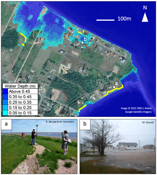
4.4 Meteorological Data

Meteorological phenomena—including storm winds, atmospheric pressure fluctuations, and precipitation—are significant, often dominant, drivers of coastal flood hazards. In regions where sea ice is prevalent, air temperature and other atmospheric parameters influence the formation and persistence of ice, which can have a knock-on effect on waves and storm surges.

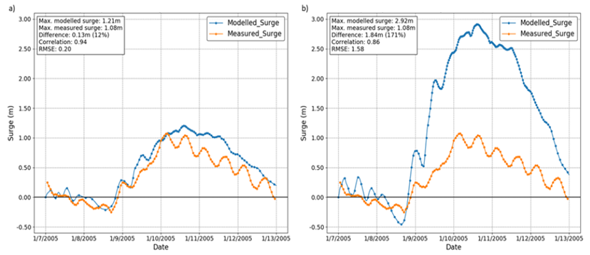
Reliable, long-term historical meteorological measurements are available for download from the Environment and Climate Change Canada (ECCC) online archives (Government of Canada, 2021c) for stations across the country. As explained by Murphy et al. (2020), there is also a variety and an increasing number of gridded atmospheric data products available from various sources, which may comprise hindcasts, reanalyses, and forecasts/nowcasts. These gridded (model-based) products are typically relied on wherever long-term measurements are unavailable, or to provide expanded spatial coverage (e.g., for use in driving numerical models of storm surge). Forecasts/nowcasts include ECCC’s High-Resolution Deterministic Prediction System, for which archived data is available at 2.5-km spatial resolution (Government of Canada, 2014). Reanalyses combine model data and observational data, and therefore typically provide more reliable multi-decadal records than hindcasts or forecasts/nowcasts, as needed to capture extreme storm events for risk-based analyses. However, trade-offs surrounding the temporal and spatial resolution of available data may affect the selection of atmospheric data products, depending on specific applications. Higher temporal and spatial resolutions are preferred for capturing the sharp gradients in atmospheric parameters associated with intense storms. Reduced skill associated with atmospheric data near land-sea interfaces is a common artifact of gridded datasets, which higher spatial resolutions can help to address. Because some gridded datasets perform better than others in different regions, it is always necessary and of crucial importance to validate gridded datasets locally using observations (e.g., Kim et al., 2021), which may guide the selection of data products for specific applications. Examples of reanalysis datasets include NOAA’s Climate Forecast System Reanalysis (CFSR) (Saha et al., 2010) and the European Centre for Medium-Range Weather Forecasts’ ERA5 Reanalysis (Hersbach et al., 2017).

An alternative (or complementary) approach to relying on gridded atmospheric datasets for numerically simulating waves and storm surges is to generate synthetic cyclone wind fields (e.g., Hardy et al., 2010). This method was traditionally required to capture strong gradients in wind and atmospheric pressure fields associated with intense tropical storms, with the synthetic storms often merged with, or inserted into, coarser-resolution gridded datasets. As the spatial and temporal resolution of reanalysis products continues to increase, it is envisaged that such techniques may not be required for Canadian applications. However, synthetic storm simulations offer possibilities to extend the historical record and support extreme value statistical analyses for particularly rare or infrequent event types (e.g., post-tropical storms in Atlantic Canada).

4.5 Water Level Data

Availability of, and access to, water level data are crucial prerequisites for coastal flood hazard assessment. Long-term water level records from tide gauges, for example, are needed to support the statistical analyses required to estimate, and assign likelihoods to, extreme water levels. In the context of risk-based storm surge flood assessment, water level data are a foundational component of the hazard scenario development. In addition, water level data are required to support model calibration and validation during the hazard assessment process. As described by Murphy et al. (2020), “Ideally, long-term measurements are available at or near the site where risks are being assessed, providing insight to short-term (e.g., tides, storm surges and seiches), seasonal (e.g., in response to hydrological cycles), interannual (e.g., driven by climate variability) and long-term (relative sea-level change) fluctuations in water levels.” Murphy et al. (2020) further describe the utility of semi-qualitative data, such as photographs, high-water marks on buildings, log and debris lines, and anecdotal information on the extent and severity of past storm and tsunami events to support analyses and supplement quantitative data (Didier et al., 2015; Environment Canada, 2006; Ferguson et al., 2022; Forbes et al., 2013; Harper et al., 1988; Kim et al., 2021; Leonard & Bednarski, 2014).

Murphy et al. (2020) provide recent and comprehensive guidance on available water level data resources, as well as considerations for data acquisition and quality control. Readers are directed to Murphy et al. (2020) for detailed guidance; however, key concepts are summarized in Box 4-5 below.

4.6 Waves

Waves can contribute significantly to coastal flood hazards in exposed open-coast settings. A first step in understanding the potential contribution to hazards is to review available offshore wave data, which may be measured/observed or model-based.

Measured wave data include wave buoy observations, available from the Marine Environmental Data Section (MEDS) archives, maintained by Fisheries and Oceans Canada (Government of Canada, 2019). Records for 565 buoys are available in the Pacific, Atlantic, and Arctic Oceans, with some buoys recording since the 1970s. However, the duration of records available for each of the buoys is highly variable. Gridded (model-based) wave data products are also available, providing expanded spatial and temporal coverage. Global reanalysis datasets, such as ECMWF Reanalysis 5^th Generation (ERA5) by the European Centre for Medium-Range Forecasts (Hersbach et al., 2017) can provide hourly wave parameters on a roughly 30-km resolution grid, covering historical periods from 1979 to the present day. Domestic hindcast products, such as MSC50 Atlantic, Northeast Pacific GROW-Fine, and Beaufort MSCB, distributed by Fisheries and Oceans Canada are available for each of Canada’s marine coastal regions (Government of Canada, 2020). The spatial and temporal resolution, and period of record, of these domestic products all vary by region.

Wave buoys operated and maintained by Fisheries and Oceans Canada are sparsely distributed in Canada’s offshore waters and generally do not provide continuous, long-term (i.e. multi-decadal, or even multi-year) records. The short duration of wave buoy deployments means the records often fail to capture more extreme (storm) events of relevance to coastal flood hazard assessment. They also tend to be located in deeper, offshore waters and, thus, do not often provide data of direct relevance to characterizing nearshore wave climates. However, in the absence of nearshore wave datasets, offshore wave buoy data may prove useful to support some calibration and validation of numerical wave models (particularly regional wave growth and transformation models), and/or to provide boundary condition input to wave transformation models (if at least some storm events are captured). Because waves transform as they propagate into nearshore waters and onshore (through processes such as shoaling, refraction, breaking, diffraction, frictional dissipation, and non-linear wave interactions), observations in nearshore and onshore areas are preferred to locally verify and quantify uncertainty in predictive wave models. However, this may require project-specific deployment of wave buoys or pressure sensors in nearshore areas (ideally across the surf zone to ensure wave transformations are captured), and/or land-based surveys of high water marks and debris/wrack lines. Both approaches to nearshore/onshore data acquisition may be challenging, time-consuming (requiring lengthy durations to capture storm events), and costly (time, labour and equipment). Lintern et al. (2024) describe methods and instruments that can be applied to support project-specific wave monitoring, as well as anticipated effort and expenses (see Table 12.4-1 of the publication). The cost-benefit and schedule impacts of project-specific wave data acquisition programs should be weighed against the expected contribution of waves to the overall coastal flood hazards (i.e. cost-benefit would be higher on open, exposed coasts), confidence/uncertainty in predictive wave models, the purpose of the hazard/risk assessment, and tolerable uncertainty in the hazard/risk assessment. Innovative techniques (e.g. radar installations, remote sensing, and machine learning-based processing of camera images) are emerging, which may help to lower the cost of nearshore wave data acquisition in the future.

More detailed information on available wave data for Canada’s coastal regions is provided by Murphy et al. (2020).

4.7 Tsunami Hazard Sources

For most communities across Canada, tsunamis are infrequent and typically not as much of a focus for flood mapping as the more frequent river and coastal flood hazards that drive land use planning and flood risk mitigation decisions. Tsunamis, however, can be generated in all three oceans bordering Canada and on lakes (seiches). In this guideline, we will consider tsunamis generated from earthquakes, both distant and local, and from landslides (both submarine and subaerial). Tsunamis can also be generated from volcanic eruptions, iceberg calving or capsizing, atmospheric conditions (meteotsunamis; Thomson et al., 2009; Mercer et al., 2002), as well as from (rare) asteroid impacts. Tsunami waves, generated by displacement of a body of water, from above or below, can occur in both marine and inland waters. A challenge in modelling tsunamis is identifying and constraining the occurrence, frequency, size, and characteristics of potential source events. In addition, as the climate changes, the effects of extreme meteorological conditions are unclear. For instance, slope failures on steep and oversteepened slopes could augment the magnitude and frequency of tsunami events. On the Arctic and Atlantic coasts, locally damaging waves can also occur from iceberg sources. Ice-borne regions should take into account the effects of seasonal hazard variations from varying sea-ice conditions.

A preliminary tsunami hazard assessment (Leonard et al., 2012) has been developed for Canada. This assessment estimates the probability of a tsunami exceeding a given wave runup height for a range of time periods for tsunamis triggered by local and far-field earthquakes, and large submarine landslide sources. The publication identifies tsunami sources for coastal regions across Canada.

A global historical tsunami database developed by the National Geophysical Data Center provides details on recorded tsunami events from 2100 BCE to the present for the Atlantic, Indian, and Pacific Oceans; and the Mediterranean and Caribbean Seas (NOAA, 2021).

4.7.1 Earthquake-Triggered Sources

Earthquake-triggered tsunamis can be complex. For instance, the recent November 2016 tsunami in New Zealand was generated by the inland magnitude (Mw) 7.8 earthquake that ruptured multiple faults under land and offshore; the offshore seafloor displacement caused a significant tsunami (Power et al., 2017). In addition, variations in how a fault ruptures can have a dramatic difference on the tsunami runup at the coast. Given the number of earthquakes recorded on the Pacific coast and around the Pacific Rim, this coastline experiences the highest risk for tsunami hazard, followed by the Atlantic coast and the Arctic coast. However, as ice coverage in the Atlantic and Arctic coastline changes, the effects of tsunamis will increase. Tsunamis triggered by significant distant earthquakes (magnitude >8) can travel long distances and take hours to reach the coastline. For these types of events, the earthquake may not be felt before the wave arrives. A series of waves generated from these events can have wavelengths of hundreds of kilometres in length and travel at high speeds. The wave trough reaches the land first, leaving the foreshore area bare of water. After some time, the waters rush inland as the crest arrives. On the other hand, a tsunami triggered by a local crustal earthquake source can result in damaging waves that arrive in minutes following the earthquake shaking. In the shoreline region, tsunami waves can produce overwash surges and backwash flow. As the wave approaches the coast, the waves erode and incorporate sediment. The advancing wave can generate considerable hydrodynamic pressures on the seafloor that result in mass soil movements and slope instabilities (Figure 4.3).

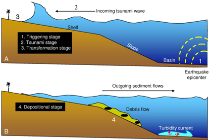
4.7.2 Thrust Earthquakes (Near and Distant)

Three major thrust fault zones occur along the Pacific coast of Canada and present potential tsunami sources, via displacement of the seafloor. These include the Cascadia subduction zone extending from southwestern British Columbia to northern California, the southern Queen Charlotte margin in the Haida Gwaii area, and the Winona Basin northeast of Vancouver Island. The Cascadia subduction zone, including the Explorer segment, presents the highest tsunami hazard to the Pacific coast, with the most extreme potential runup along the outer southern coast of British Columbia and a lesser danger in the inner Pacific coasts of Juan de Fuca and Georgia Straits. Along the northern BC coastline, the transpressive Queen Charlotte margin contributes to a significant proportion of the tsunami hazard. Potential rupture geometries for a magnitude 9 Cascadia subduction megathrust tsunami source include buried, splay-faulting, and trench-breaching rupture scenarios that can be found in Gao et al. (2018), with slight updates for southernmost Cascadia in the Master’s thesis of Sypus (2019). The Winona Basin area just north of the Cascadia subduction zone may also have the potential to host a tsunamigenic thrust earthquake; rupture scenarios are provided by Sypus (2019), but due to the challenges in constraining uncertainties in the tectonics of the area it has not been included in formal hazard assessments. In 2012, a magnitude 7.8 earthquake just off the coast of Haida Gwaii resulted in a large tsunami (Leonard & Bednarski, 2014; 2015; Fine et al., 2015). This event demonstrated the presence of a previously poorly known and poorly constrained (e.g., Leonard et al., 2012) subduction megathrust with the capacity for tsunamigenic rupture. Candidate tsunami sources have been developed for this fault, including buried and trench-breaching ruptures. These scenarios include long ruptures from mid-way between Haida Gwaii and Vancouver Island to mid-way between Haida Gwaii and the southern tip of Alaska Panhandle and shorter rupture scenarios north and south of the main rupture of the 2012 earthquake (Sypus, 2019).

Far-field subduction zone sources contribute to the tsunami hazard on the Pacific and Atlantic coast. The tsunami hazard on the Arctic coastline, however, remains poorly constrained. In the Pacific, the two largest and most damaging recorded tsunamigenic megathrust earthquakes occurred in Alaska (Mw 9.2, 1964) and Chile (Mw 9.5, 1960); the 1964 tsunami caused considerable damage on the west coast of Vancouver Island, including Port Alberni (White, 1966).

4.7.3 Crustal Earthquakes

Rupture of submarine crustal faults may trigger locally damaging waves by coseismic displacement of the seafloor. Crustal faults host smaller magnitude earthquakes than those at plate boundaries and can be expected to generate smaller tsunami waves. For these types of tsunamis, there may be little wave attenuation and short warning times between the onset of ground shaking and the arrival of damaging waves. Compared to the megathrust sources, the recurrence interval of the crustal events is expected to be very long and their source models generally have greater uncertainties. Source models have been developed for a number of crustal faults in the Strait of Georgia region that have recently been identified as active (Caston, 2021).

4.7.4 Landslide Events

Landslide-triggered tsunamis can be caused by failure of steep subaerial slopes or submarine delta fronts, resulting from earthquake-triggered ground shaking, rainfall, construction, or other factors. In some cases, failures can occur months to years after significant seismic activity (e.g., Goff & Sugawara, 2014). Oversteepened fiord slopes and the leading edge of submarine deltas are areas of particular concern (e.g., Mosher, 2009). The ground motion from an earthquake affects the soil cyclically and may reduce the shear strength of the soil (Duncan & Wright, 2005).

The displacement of water by a landslide may cause extremely large tsunami waves (e.g., the 525-m runup in 1958 Lituya Bay tsunami in Alaska; Miller, 1960), but impacts are generally more localized than for tsunamis triggered directly by earthquake displacements of the seafloor. Many parts of the Canadian coastline are susceptible to landsliding with the potential to generate damaging waves, but the history of past events and their impacts are poorly known (e.g., Leonard et al., 2012). Examples of damaging events in Canada include tsunamis triggered by: a subaerial rock avalanche in Knight Inlet, BC, that destroyed a First Nations village in the 1600s (Bornhold et al., 2007), a submarine failure in Kitimat Arm, BC, in 1975 (Skvortsov & Bornhold, 2007), and a submarine continental slope failure at the Grand Banks offshore of Newfoundland that caused 28 fatalities in 1929 (e.g., Fine et al., 2005). Landslides commonly occur repeatedly at particular sites, so mapping of landslide deposits may be an indication of future hazard; efforts are underway to compile a national database of submarine landslide deposits (Lintern et al., 2020).

4.7.5 Paleotsunami Data

The age and relative elevation of tsunami deposits preserved in coastal sediment sequences provide important constraints on the size and frequency of past events; the NCEI/WDS (n.d.) Tsunami Deposit Database provides a useful global compilation. A caveat is that the distribution of tsunami deposits rarely reflects the full impact of a tsunami; tsunamis do not always leave sediment deposits, and the deposits are often poorly preserved (e.g., Szczucinski, 2011; Leonard & Bednarski, 2015). Oral histories from coastal First Nations (e.g., Ludwin et al., 2005) in combination with paleotsunami, paleoseismic, and/or archaeological studies can help to provide further constraints. A detailed compilation and interpretation of paleotsunami data for the Pacific coast of Canada is provided by Goff et al. (2020). A recent review of tsunami deposits around the entire Atlantic Ocean basin (Costa et al., 2021) includes only one deposit in Canada, from the 1929 Grand Banks event.

Studies to match paleo-source and paleotsunami records can help to validate the earthquake/landslide and tsunami sources, and to refine average recurrence intervals. Evidence of abrupt coastal land-level change due to fault rupture, as might be recorded by a change between freshwater and saline indicators in a sediment sequence, is often coincident with a tsunami deposit (e.g., Atwater et al., 2005). Studies of paleo-landslide tsunami events may be aided by matching the age of landslide deposits on the seafloor with evidence of onshore tsunami inundation, or potentially with seafloor erosional features (e.g., Bornhold et al., 2007; Greene et al., 2018). The recurrence of Cascadia subduction megathrust events is constrained largely from the offshore record of turbidite deposits, inferred to be caused by concurrent triggering of turbidity currents at the heads of submarine canyons along the margin during strong shaking over a wide region (e.g., Goldfinger at al., 2012).

4.8 Sea Ice Data

The Canadian Ice Service (CIS), a branch of Environment and Climate Change Canada, has been recording and producing regional ice charts since 1968. Latest ice conditions and historical data are available online (Government of Canada, 2021d). Regions that have records include the Western Arctic, the Eastern Arctic, Hudson Bay, the Gulf of St.-Lawrence, the Great Lakes, Newfoundland, the High Arctic, Waterways, and the Arctic Ocean. Daily ice charts have been produced since 1999, while weekly ice charts have been produced since 1968. Black and white and WMO (World Meteorological Organization) colour charts are available. Ice charts from the CIS are ESRI (Environmental Systems Research Institute), predominantly ArcInfo interchange files (e00), and require conversion to another file format for ease of use. Parameters, such as total concentration, state of development, ice thickness, and form of ice, are displayed in the CIS ice charts. The National Snow and Ice Data Center (NSIDC), run by the University of Colorado Boulder Cooperative Institute of Research, provides global sea ice data through processed datasets (National Snow and Ice Data Center, 2019). These data are often supplied in common file formats (e.g., shapefiles or GeoTIFFs) and can provide an easy and quick look at the long-term trends in sea ice presence. Currently, robust and publicly available data of measurements for individual ice floes are not available. Thus, a more in-depth analysis of the air-ice-ocean momentum exchange is difficult to perform during coastal hazard assessments.

4.9 Land Cover and Roughness

Hydrodynamic models require input regarding the land surface and ocean floor roughness in order to drive computational processes that simulate friction between the surfaces and the water. Roughness depends, in part, on the surficial material, as well as vegetation. For example, smooth surfaces, such as paved concrete or asphalt, will exert less friction on the flow than rough surfaces composed of coarse granular material or vegetated earth. Roughness may also vary at a given location owing to seasonal changes in surface conditions and vegetation (Arcement & Schneider, 1989). Roughness parameterization is comparatively more important in locations where shallow flows are anticipated (e.g. where overland flooding is anticipated) and less important for deep, offshore locations where roughness has only a small influence on the hydraulics.

Roughness is often represented using the Manning’s n coefficient (Arcement & Schneider, 1989; Chow, 1959). In general, practitioners must use engineering judgement to identify initial estimates for roughness coefficients based on knowledge of the land cover and vegetation. An abundance of engineering guides and resources are available to assist practitioners in selecting Manning’s n roughness coefficients (Arcement & Schneider, 1989; Chin, 2013; Chow, 1959; Houghtalen et al., 2010). Often, roughness coefficients are treated as a calibration parameter and are adjusted during the model calibration process to optimize model performance.

A number of resources are available to assist practitioners in understanding the type of land cover present at a given location. Some jurisdictions may maintain geospatial products (e.g., maps or GIS databases) illustrating the distribution of relevant information, such as land use or vegetation type. For example, the Government of New Brunswick maintains geospatial databases illustrating the distribution of forested, non-forested, and wetland areas, further categorizing non-forested areas by vegetation type including: no vegetation; grasses, crops, or other; shrubs; or trees (Department of Environment and Local Government, 2019; Department of Natural Resources, 2019a, 2019b). Satellite imagery, photography, and video products may also be used to enhance understanding of land cover; however, practitioners must be attentive to the dates associated with these types of products to evaluate relevance to the study. In-person site visits may also be leveraged to evaluate land cover.

4.10 Buildings, Infrastructure, and Flood Defences

In developed areas, practitioners may need to consider the impacts of infrastructure on the propagation of floodwaters and hazard pathways (see Section 5.2.2). For example, infrastructure, such as buildings, walls, roads, and flood defences, may obstruct flow and/or attenuate wave effects, whereas drainage infrastructure (e.g., culverts) may facilitate flood propagation across connected land parcels. Depending on the level of post-processing, these features may or may not be reflected in the elevation datasets that will be used to support flood modelling and associated analyses; digital elevation models (DEMs) often illustrate a bare-earth representation of the earth surface, whereas digital surface models (DSMs) or raw lidar data illustrate the elevation of the bare-earth surface plus any surficial coverings, such as buildings or vegetation (Zhou, 2017).

Statistics Canada’s Open Database of Buildings (ODB) is a collection of open data on buildings, primarily building footprints, based on publicly available municipal, regional, or provincial data sources (Statistics Canada, 2020). The ODB contains geospatial data depicting building footprints, as well as attribute data summarizing key geospatial and administrative information, including geographic coordinates, area, perimeter, data provider, census subdivision unique identifier, and census subdivision name. Where building data are not available from the ODB, or where additional detail is required, practitioners are encouraged to investigate availability from municipal, regional, or provincial governments or institutions. Similarly, information regarding flood defences and drainage infrastructure may require a special request to local governing bodies or institutions.

4.11 Climate Change Projections

4.11.1 Climate Change – Sea Ice

The Arctic sea-ice environment has changed significantly over recent decades (Barber et al., 2017). Perennial sea ice that survives the summer melt is being replaced by thinner seasonal sea ice that melts in the summer. Summer sea-ice area (particularly multi-year ice—MYI) declined across the Canadian Arctic by 5% to 20% per decade (1968–2016, depending on region); winter sea-ice area decreased in eastern Canada by 7.6% per decade (1969–2016) (Derksen et al., 2019). It is very likely that continued reductions in summer and fall sea ice across the Canadian Arctic, and winter sea ice in eastern Canadian waters, will result from increased temperatures under all future emissions scenarios. Most Canadian Arctic marine regions could be sea ice–free for at least one month in the summer by 2050 based on simulations from CMIP5 models. There is very high confidence that the region to the north of the Canadian Arctic Archipelago (CAA) and Greenland will be the last area where thick MYI will be present in the Arctic during the summer.

4.11.2 Climate Change Marine Winds and Waves

Consistent significant trends in winds, storminess, and waves have not been found for most of the waters off Canada, in part due to limited data and strong effects of natural variability. Long-term data are minimal, have a very coarse spatial resolution, and do not cover nearshore areas. A slight northward shift of storm tracks, with decreased wind speed and lower wave heights off Atlantic Canada, has been observed and is projected to continue. Off the Pacific coast, wave heights have been observed to increase in winter and decrease in summer, and these trends are projected to continue in future. Surface wave heights and the duration of the wave season in the Canadian Arctic have increased since 1970 and are projected to continue to increase over this century as sea ice declines. Off Canada’s east coast, areas that currently have seasonal sea ice are also anticipated to experience increased wave activity in the future, as seasonal ice duration decreases (Greenan et al., 2019).

4.12 Sea-Level Change for the Oceans Surrounding Canada

Global mean sea-level (GMSL) change is occurring on temporal and spatial scales that threaten coastal communities, cities, and low-lying islands. GMSL has increased by 0.20 [0.15 to 0.25] m between 1901 and 2018 (IPCC, 2021). The average rate of sea-level rise was 1.3 [0.6 to 2.1] mm yr–¹ between 1901 and 1971, increasing to 1.9 [0.8 to 2.9] mm yr–¹ between 1971 and 2006, and further increasing to 3.7 [3.2 to 4.2] mm yr–¹ between 2006 and 2018.

It is virtually certain that the global mean sea level will continue to rise over the 21st century (IPCC, 2021). Relative to 1995–2014, the likely GMSL rise by 2100 is 0.28–0.55 m under the very low greenhouse gas (GHG) emissions scenario (SSP1-1.9), 0.32–0.62 m under the low GHG emissions scenario (SSP1-2.6), 0.44–0.76 m under the intermediate GHG emissions scenario (SSP2-4.5), and 0.63–1.01 m under the very high GHG emissions scenario (SSP5-8.5). GMSL rise above the likely range—approaching 2 m by 2100 and 5 m by 2150 under a very high GHG emissions scenario (SSP5-8.5) (low confidence)—cannot be ruled out due to deep uncertainty in ice sheet processes.

At coastal locations, the sea-level change that is experienced relative to land is known as “relative” sea-level change; this can differ from absolute sea-level change because of geophysical and geological processes that cause land to move upward (“uplift”) or downward (“subsidence”). The long-term trends in relative sea-level observed at tide gauges in Canada vary substantially from one location to another. Some of the variability is due to oceanographic factors affecting the absolute elevation of the sea surface, but a major determinant of relative sea-level change in Canada is vertical land motion. Land subsidence (sinking) increases relative sea level, while land uplift does the opposite. Across much of Canada, land uplift or subsidence is mainly due to the delayed effects of the last continental glaciation (ice age), called glacial isostatic adjustment (GIA). GIA is still causing uplift of the North American continental crust in areas close to the centre of former ice sheets, such as Hudson Bay, and subsidence in regions on the edge of former ice sheets, such as the southern part of Atlantic Canada. On the west coast, active tectonics and, on the Fraser delta, sediment consolidation contributes to vertical land motion. In areas with earthquake activity, incorporation of tectonic uplift to reduce relative sea level rise under future scenarios, as well as the potential for post-seismic relaxation in certain areas could be considered.

Projections of future changes in relative sea level include the effects of changes in glacier and ice-sheet mass loss, thermal expansion of the oceans, changing ocean circulation conditions, and human-caused changes in land water storage. Vertical land motion is a very important element of relative sea-level change for Canada’s coastline. James et al. (2021) describe relative sea-level projections based on IPCC AR5 projections with an improved land motion model developed by the Canadian Geodetic Survey (Robin et al., 2020; Canadian Geodetic Survey, 2019). The CGS model was developed to replace the less-accurate land motion values utilized by the IPCC AR5.

4.13 References

Arcement, G. J. & Schneider, V. R. (1989). Guide for Selecting Manning’s Roughness Coefficients for Natural Channels and Flood Plains. Water-Supply Paper. U.S. Geological Survey

Atwater, B. F., Musumi-Rokkaku, S., Satake, K., Tsuji, Y., Ueda, K., & Yamaguchi, D.K. (2005). The orphan tsunami of 1700 - Japanese clues to a parent earthquake in North America. University of Washington Press.

Barber, D. G., Meier, W. N., Gerland, S., Mundy, C. J., Holland, M., Kern, S., Li, Z., Michel, C., Perovich, D. K., Tamura, T., Berge, J., Bowman, J., Christiansen, J. S., Ehn, J. K., Ferguson, S., Granskog, M. A., Kikuchi, T., Kuosa, H., Light, B., … Zhang, L. (2017). Arctic Sea Ice; in Snow Water Ice and Permafrost in the Arctic (SWIPA), Arctic Monitoring and Assessment Programme (AMAP), Oslo, Norvège, 103–136.

Bedford Institute of Oceanography. (2020). WebTide Tidal Prediction Model. https://www.bio.gc.ca/science/research-recherche/ocean/webtide/index-en.php

Bernier, N. (2005). Annual and Seasonal Extreme Sea Levels in the Northwest Atlantic: Hindcasts Over the Last 40 Years and Projections for the Next Century. [Doctoral Thesis, Dalhousie University]. DalSpace.

Bornhold, B. D., Harper, J. R., McLaren, D., & Thomson, R. E. (2007). Destruction of the First Nations village of Kwalate by a rock avalanche-generated tsunami. Atmosphere-Ocean, 45(2), https://doi.org/10.3137/ao.450205.

British Columbia Ministry of Environment. (2009). Manual of British Columbia Hydrometric Standards (Version 1.0).

Canadian Geodetic Survey. (2019). NAD83(CSRS) v7. https://webapp.geod.nrcan.gc.ca/geod/tools-outils/nad83-docs.php

Caston, M. (2021). Tsunamigenic potential of crustal faults in the southern Strait of Georgia and Boundary Bay. [Master’s thesis, University of Victoria].

Chin, D. A. (2013). Water Resources Engineering (3rd Edition). Pearson Education Inc.

Chow, V. T. (1959). Open-Channel Hydraulics. McGraw-Hill Book Company Inc.

CHS. (2018). Canadian Hydrographic Service Non-Navigational (NONNA) Bathymetric Data. https://open.canada.ca/data/en/dataset/d3881c4c-650d-4070-bf9b-1e00aabf0a1d

Codiga, D. L. (2011). Unified Tidal Analysis and Prediction Using the UTide Matlab Functions (Technical Report 2011-01). Graduate School of Oceanography, University of Rhode Island. ftp://www.po.gso.uri.edu/ pub/downloads/codiga/pubs/2011Codiga-UTide-Report.pdf

Costa P. J. M., Dawson, S., Ramalho, R. S., Engel, M., Dourado, F., Bosnic, I., & Andrade, C. (2021). A review on onshore tsunami deposits along the Atlantic coasts. Earth-Science Reviews, 212(103441), https://doi.org/10.1016/j.earscirev.2020.103441

Murphy, E., Cornett, D. Van Proosdij, D., & Mulligan, R.P. (2024). Nature-based infrastructure for coastal flood and erosion risk management: a Canadian design guide. National Research Council of Canada. Ocean, Coastal and River Engineering, 348 p. https://doi.org/10.4224/40003325

Province of New Brunswick. (2019). geonb_wetlands-terreshumides—ESRI Shape File. http://www.snb.ca/geonb1/e/DC/catalogue-E.asp

Province of New Brunswick. (2019a). geonb_forest-foret—ESRI Shape File. http://www.snb.ca/geonb1/e/DC/catalogue-E.asp

Province of New Brunswick. (2019b). geonb_nonforest-nonforet—ESRI Shape File. http://www.snb.ca/geonb1/e/DC/catalogue-E.asp

Derksen, C., Burgess, D., Duguay, C., Howell, S., Mudryk, L., Smith, S., Thackeray, C. & Kirchmeier-Young, M. (2019). Changes in snow, ice, and permafrost across Canada. In Bush, E. & Lemmen, D.S. (Eds.), Canada’s Changing Climate Report (pp. 194-260). Gouvernement du Canada. https://changingclimate.ca/CCCR2019/

DHI. (2017). MIKE 21 Tidal Analysis and Prediction Module Scientific Documentation.

Didier, D., Bernatchez, P., Boucher-Brossard, G., Lambert, A., Fraser, C., Barnett, R., & Van-Wierts, S. (2015). Coastal Flood Assessment Based on Field Debris Measurements and Wave Runup Empirical Model. Journal of Marine Science and Engineering, 3(3), 560–590, https://doi.org/10.3390/jmse3030560

Duncan, J. M., & Wright, S. G. (2005). Soil Strength and Slope Stability (1st ed.). Wiley.

Eakins, B. W., & Grothe, P. R. (2014). Challenges in Building Coastal Digital Elevation Models. Journal of Coastal Research, 297(5), 942–953. https://doi.org/10.2112/jcoastres-d-13-00192.1

Eakins, B. W., Danielson, J. J., Sutherland, M. G., & Mclean, S. J. (2015). A framework for a seamless depiction of merged bathymetry and topography along U.S. coasts. [Conference]. U.S. HYDRO Conference Proceedings.

Egbert, G. D., & Erofeeva, S. Y. (2002). Efficient Inverse Modeling of Barotropic Ocean Tides. Journal of Atmospheric and Ocean Technology, 19, 183–204.

Environment Canada. (2006). Impacts of Sea-Level Rise and Climate Change on the Coastal Zone of Southeastern New Brunswick. https://publications.gc.ca/site/eng/9.683399/publication.html

Ferguson, S., Provan, M., Murphy, E., Bérubé, D., Desrosiers, M., Robichaud, A., & Kim, J. (2022). Assessing numerical model skill at simulating coastal flooding using field observations of deposited debris and photographic evidence. Water, 14(4), 589. https://doi.org/10.3390/w14040589

Fine, I. V., Cherniawsky, J. Y., Thomson, R. E., Rabinovich, A. B., & Krassovski, M. V. (2015). Observations and numerical modeling of the 2012 Haida Gwaii tsunami off the coast of British Columbia. Pure and Applied Geophysics, 172, 699-718. https://doi.org/10.1007/s00024-014-1012-7.

Fine, I. V., Rabinovich, A. B., Bornhold, B. D., Thomson, R. E. & Kulikov, E. A. (2005). The Grand Banks landslide-generated tsunami of November 18, 1929: preliminary analysis and numerical modeling. Marine Geology, 215, 45-57.

Fisheries and Oceans Canada. (2021). Fisheries and Oceans Canada in the Pacific Region. https://www.pac.dfo-mpo.gc.ca/index-eng.html

Fisheries and Oceans Canada. (2022). Tides, Currents, and Water Levels. Retrieved October 22, 2024. https://www.tides.gc.ca/

Forbes, D. L., Whalen, D., Jacobson, B., Fraser, P., Manson, G., Couture, N., & Simpson, R. (2013). Co-design of coastal risk analysis for subsistence infrastructure in the Inuvialuit Settlement Region, western Arctic Canada. [Poster]. ArcticNet Annual Scientific Meeting, Halifax, NS.

Foreman, M. G. G. (1977). Manual for tidal heights analysis and prediction (Pacific Marine Science Report 77-10). Institute of Ocean Sciences.

Gao, D., Wang, K., Insua, T. L., Sypus, M., Riedel, M., & Sun, T. (2018). Defining megathrust tsunami source scenarios for northernmost Cascadia. Natural Hazards, 94, 445–469. https://doi.org/10.1007/s11069-018-3397-6

GEBCO. (2020a). GEBCO Overview. https://www.gebco.net/about_us/overview/

GEBCO. (2020b). GEBCO_2019 Grid. https://www.gebco.net/data_and_products/gridded_bathymetry_data/gebco_2019/gebco_2019_info.html

GEBCO. (2020c). GEBCO_2020 Grid. https://www.gebco.net/data_and_products/gridded_bathymetry_data/gebco_2020/

Goff, J. & Sugawara, D. (2014). Seismic driving of sand beach ridge formation in northern Honshu, Japan? Marine Geology, 358, 138-149. https://doi.org/10.1016/j.margeo.2014.04.005

Goff, J., Bobrowsky, P., Huntley, D., Sawai, Y., & Tanagawa, K. (2020). Paleotsunamis along Canada’s Pacific coast. Quaternary Science Reviews, 237(106309), https://doi.org/10.1016/j.quascirev.2020.106309

Goldfinger, C., Nelson, C. H., Morey, A. E., Johnson, J. E., Patton, J. R., Karabanov, E. B., Gutierrez-Pastor, J., Eriksson, A. T., Gracia, E., Dunhill, G., Enkin, R. J., Dallimore, A. & Vallier, T. (2012). Turbidite event history - Methods and implications for Holocene paleoseismicity of the Cascadia subduction zone. U.S. Geological Survey Professional Paper 1661-F. https://doi.org/10.3133/pp1661F

Government of Canada. (2014). High Resolution Deterministic Prediction System. https://data.ec.gc.ca/data/weather/products/high-resolution-deterministic-prediction-system/

Government of Canada. (2019). Canadian Wave Data. https://meds-sdmm.dfo-mpo.gc.ca/isdm-gdsi/waves-vagues/index-eng.htm

Government of Canada. (2020). MSC50 Wind and Wave Climate Hindcast. https://www.isdm-gdsi.gc.ca/isdm-gdsi/waves-vagues/MSC50-eng.html

Government of Canada. (2021a). Geodetic tools and data. https://www.nrcan.gc.ca/maps-tools-and-publications/tools/geodetic-reference-systems/data/10923

Government of Canada. (2021b). GPS·H. https://webapp.geod.nrcan.gc.ca/geod/tools-outils/gpsh.php

Government of Canada. (2021c). Historical Climate Data. https://climate.weather.gc.ca/

Government of Canada. (2021d). Latest ice conditions. https://www.canada.ca/en/environment-climate-change/services/ice-forecasts-observations/latest-conditions.html

Government of Canada. (2021e). Passive Control Networks. https://webapp.geod.nrcan.gc.ca/geod/data-donnees/passive-passif.php?locale=en

Greenan, B. J. W., James, T. S., Loder, J. W., Pepin, P., Azetsu-Scott, K., Ianson, D., Hamme, R. C., Gilbert, D., Tremblay, J-E., Wang, X. L. & Perrie, W. (2019). Changes in oceans surrounding Canada. In Bush, E. & Lemmen, D.S. (Eds.), Canada’s Changing Climate Report (pp. 343-423). Government of Canada. https://changingclimate.ca/CCCR2019/

Greene, H. G., Barrie, J. V., & Todd, B. J. (2018). The Skipjack Island fault zone: An active transcurrent structure within the upper plate of the Cascadia subduction complex. Sedimentary Geology, 378, 61-79. https://doi.org/10.1016/j.sedgeo.2018.05.005

Hardy T. A., Mason L. B., & McConochie J. D. (2010). Generating Synthetic Tropical Cyclone Databases for Input to Modeling of Extreme Winds, Waves, and Storm Surges. In Charabi Y. (Ed.) Indian Ocean Tropical Cyclones and Climate Change. Springer. https://doi.org/10.1007/978-90-481-3109-9_9

Harper, J. R., Henry, R. F., & Stewart, G. G. (1988). Maximum storm surge elevations in the Tuktoyaktuk region of the Canadian Beaufort Sea. Arctic, 41(1), 48–52.

Hersbach, H., Bell, B., Berrisford, P., Hirahara, S., Horányi, A., Muñoz‐Sabater, J., Nicolas, J., Peubey, C., Radu, R., Schepers, D., Simmons, A., Soci, C., Abdalla, S., Abellan, X., Balsamo, G., Bechtold, P., Biavati, G., Bidlot, J., … Thépaut, J-N. (2017). Complete ERA5 from 1940: Fifth generation of ECMWF atmospheric reanalyses of the global climate. Copernicus Climate Change Service. https://doi.org/10.24381/cds.143582cf

Houghtalen, R. J., Akan, A. O., & Hwang, N. H. C. (2010). Fundamentals of Hydraulic Engineering Systems (4th Ed). Prentice Hall.

Intergovernmental Oceanographic Commission. (2016). Manual on Sea-Level Measurements and Interpretation, Volume V: Radar Gauges (JCOMM Technical Report No. 89).

IPCC. (2021). Summary for Policy makers. Dans Masson-Delmotte, V., P. Zhai, A. Pirani, S.L. Connors, C. Péan, S. Berger, N. Caud, Y. Chen, L. Goldfarb, M.I. Gomis, M. Huang, K. Leitzell, E. Lonnoy, J.B.R. Matthews, T.K. Maycock, T. Waterfield, O. Yelekçi, R. Yu, & B. Zhou (Eds.) Climate Change 2021: The Physical Science Basis. Contribution of Working Group I to the Sixth Assessment Report of the Intergovernmental Panel on Climate Change. Sous presse. https://www.ipcc.ch/report/ar6/wg1/chapter/summary-for-policymakers/

James, T. S., Robin, C., Henton, J. A., & Craymer, M. (2021). Relative Sea-level Projections for Canada based on the IPCC Fifth Assessment Report and the NAD83v70VG National Crustal Velocity Model. Natural Resources Canada. https://doi.org/10.4095/327878

Kim, J., Murphy, E., Nistor, I., Ferguson, S., & Provan, M. (2021). Numerical Analysis of Storm Surges on Canada’s Western Arctic Coastline. Journal of Marine Science and Engineering, 9(3), 326. https://doi.org/10.3390/jmse9030326

Leonard, L. J., & Bednarski, J. M. (2014). Field survey following the 28 October 2012 Haida Gwaii Tsunami. Pure and Applied Geophysics, 171, 3467–3482.

Leonard, L. J., & Bednarski, J. M. (2015). The preservation potential of coastal coseismic and tsunami evidence observed following the 2012 Mw 7.8 Haida Gwaii thrust earthquake. Bulletin of the Seismological Society of America, 105(2B), 1280-1289, https://doi.org/10.1785/0120140193

Leonard, L. J., Rogers, G. C., & Mazzotti, S., (2012). A preliminary tsunami hazard assessment of the Canadian coastline (Geological Survey of Canada, Open File 7201). Natural Resources Canada. https://doi.org/10.4095/292067

Lintern, D. G., Rutherford, J., Hill, P. R., Campbell, C., & Normandeau, A. (2020). Towards a national-scale assessment of the subaqueous mass movement hazard in Canada. Geological Society, London, Special Publications, 500, p. 97-113, https://doi.org/10.1144/SP500-2019-206

Lintern, D. G., Van Proosdij, D., Manson, G., Mulligan, R., Côté, M. & Thurston, E. (2024). Chapter 12: Field Monitoring. In Murphy, E., Cornett, A., van Proosdij, D., & Mulligan, R. P. (Eds.) Nature-Based Infrastructure for Coastal Flood and Erosion Risk Management – A Canadian Design Guide. ISBN 978-0-660-71886-6.

Ludwin, R. S., Dennis, R., Carver, D., McMillan, A. D., Losey, R., Clague, J., Jonientz-Trisler, C., Bowechop, J., Wray, J., & James, K. (2005). Dating the 1700 Cascadia earthquake: great coastal earthquakes in Native stories. Seismological Research Letters, 76(2), 140-148.

Mercer, D., Sheng, J., Greatbatch, R. J., & Bobanovic, J. (2002). Barotropic waves generated by storms moving rapidly over shallow water. Journal of Geophysical Research, 107(C10), 3152. https://doi.org/10.1029/2001JC001140

Miller, D. J. (1960). The Alaska earthquake of July 10, 1958: giant wave in Lituya Bay. Bulletin of the Seismological Society of America, 50(2), 253-266.

Mosher, D. C. (2009). Submarine landslides and consequent tsunamis in Canada. Geoscience Canada, 36(4), 179-190.

Murphy, E., Cornett, D. Van Proosdij, D., & Mulligan, R.P. (2024). Nature-based infrastructure for coastal flood and erosion risk management: a Canadian design guide. National Research Council of Canada. Ocean, Coastal and River Engineering, 348 p. https://doi.org/10.4224/40003325

Murphy, E., Lyle, T., Wiebe, J., Hund, S. V., Davies, M., & Williamson, D. (2020). Coastal Flood Risk Assessment Guidelines for Building and Infrastructure Design Applications (CRBCPI-Y5-R2). National Research Council Canada.

National Snow and Ice Data Center. (2019). NSIDC Scientific Data Search. Scientific Data Search—Sea Ice. https://nsidc.org/data/search/#keywords=sea+ice/sortKeys=score,,desc/facetFilters=%257B%257D/pageNumber=1/itemsPerPage=25

National Geophysical Data Center / World Data Service: NCEI/WDS. (n.d.). Global Tsunami Deposit Database. NOAA National Centers for Environmental Information. https://www.ngdc.noaa.gov/hazel/view/hazards/tsunami/deposit-search/

National Geophysical Data Center/World Data Service: NCEI/WDS (2021). Global Historical Tsunami Database, 2100 BC to Present. NOAA National Centers for Environmental Information. https://data.noaa.gov/metaview/page?xml=NOAA/NESDIS/NGDC/MGG/Hazards/iso/xml/G02151.xml&view=getDataView [10 août 2021]

Natural Resources Canada. (2019a). High Resolution Digital Elevation Model (HRDEM) CanElevation Series Product Specifications (Ed. 1.3).

Natural Resources Canada. (2019b). Federal Geomatics Guidelines for Flood Mapping (General Information Product 114e).

Natural Resources Canada. (2020). Federal Airborne Lidar Data Acquisition Guideline (Version 3.0, General Information Product 117e). Government of Canada.

Pawlowicz, R., Beardsley, B., & Lentz, S. (2002). Classical tidal harmonic analysis including error estimates in MATLAB using T_TIDE. Computers & Geosciences, 28(8), 929–937.

Power, W., Clark, K., King, D. N., Borrero, J., Howarth, J., Lane, E. M., Goring, D., Goff, J., Chagué-Goff, C., Willimas, J., Reid, C., Whittaker, C., Mueller, C., Williams, S., Hughes, M.W., Hoyle, J., Bind, J., Strong, D., Litchfield, N. & Denson, A. (2017). Tsunami runup and tide-gauge observations from the 14 November 2016 M7.8 Kaikōura earthquake, New Zealand. Pure and Applied Geophysics, 174, 2457-2473. https://doi.org/10.1007/s00024-017-1566-2

Richards, W., & Daigle, R. (2011). Scenarios and Guidance for Adaptation to Climate Change and Sea-Level Rise—NS and PEI Municipalities. Nova Scotia Department of Environment & Atlantic Canada Adaptation Solutions Association.

Robin, C., Nudds, S., MacAulay, P., Godin, A., De Lange Boom, B., & Bartlett, J. (2016). Hydrographic vertical separation surfaces (HyVSEPs) for the tidal waters of Canada. Marine Geodesy, 39, 195–222. https://doi.org/10.1080/01490419.2016.1160011

Robin, C. M. I., Craymer, M., Ferland, R., James, T. S., Lapelle, E., Piraszewski, M., & Zhao, Y. (2020). NAD83v70VG: A new national crustal velocity model for Canada (Geomatics Canada, Open File, 62, 70). Natural resources Canada. https://doi.org/10.4095/327592

Saha, S., Moorthi, S., Pan, H.L., Wu, X., Wang, J., Nadiga, S., Tripp, P., Kistler, R., Woollen, J., Behringer, D. & Liu, H. (2010). The NCEP climate forecast system reanalysis. Bulletin of the American Meteorological Society, 91(8), 1015-1058.

Shanmugam, G. (2021). Chapter 7: Triggering mechanisms of downslope processes. In Shanmugam, G. Mass Transport, Gravity Flows, and Bottom Currents (pp. 273-307). https://doi.org/10.1016/B978-0-12-822576-9.00007-2

Skvortsov, A., & Bornhold, B. (2007). Numerical simulation of the landslide-generated tsunami in Kitimat Arm, British Columbia, Canada, 27 April 1975. Journal of Geophysical Research, 112(F2).https://doi.org/10.1029/2006JF000499

Statistics Canada. (2020). The Open DataBase of Buildings. https://www.statcan.gc.ca/eng/lode/databases/odb

Sypus, M. (2019). Models of Tsunamigenic Earthquake Rupture Along the West Coast of North America. [Master’s thesis, University of Victoria]. http://hdl.handle.net/1828/11436

Szczucinski, W. (2011). The post-depositional changes of the onshore 2004 tsunami deposits on the Andaman Sea coast of Thailand. Natural Hazards, 60, 115-133. https://doi.org/10.1007/s11069-011-9956-8

Thomson, R. E., Rabinovich, A. B., Fine, I. V., Sinnott, D. C., McCarthy, A., Sutherland, N. A. S., & Neil, L. K. (2009). Meteorological tsunamis on the coasts of British Columbia and Washington. Physics and Chemistry of the Earth, 34(17-18), 971-988. https://doi.org/10.1016/j.pce.2009.10.003

White, W.R.H. (1966). The Alaska earthquake - its effect in Canada. Canadian Geographical Journal, 72(6), 210-219.

Zhai, L., Greenan, B., Thomson, R., & Tinis, S. (2019). Use of Oceanic Reanalysis to Improve Estimates of Extreme Storm Surge. Journal of Atmospheric and Oceanic Technology, 36(11), 2205–2219.

Zhang, H., & Sheng, J. (2013). Estimation of extreme sea levels over the eastern continental shelf of North America. Journal of Geophysical Research, 118, 1–21. https://doi.org/10.1002/2013JC009160

Zhou, Q. (2017). Digital elevation model and digital surface model. In Richardson, D., Castree, N., Goodchild, M. F., Kobayashi, A., Liu, W. & Marston, R. A. (Eds.). The International Encyclopedia of Geography: People, the Earth, Environment and Technology. Wiley.

5.0 Coastal Flood Hazard Modelling and Analysis

Lead Authors

Enda Murphy (National Research Council Canada), Sean Ferguson (National Research Council Canada), Joseph Kim (University of Ottawa), Richard Thomson (Fisheries and Oceans Canada), Reza Amouzgar (Ocean Networks Canada), Thomas James (Natural Resources Canada), Isaac Fine (Fisheries and Oceans Canada), and Blair Greenan (Fisheries and Oceans Canada)

Contributors

Nicky Hastings (Natural Resources Canada) and Julie Van de Valk (Natural Resources Canada)

Suggested Citation

Murphy, E., Ferguson, S., Kim, J., Thomson, R., Amouzgar, R., James, T., Fine, I., and Greenan, B. (2025). Coastal Flood Hazard Modelling and Analysis. In Ferguson, S., Hastings, N. L., Van de Valk, J., Murphy, E. & Kim J. (Eds.) Coastal Flood Hazard Assessment for Risk-Based Analysis on Canada's Marine Coasts. Government of Canada.

5.1 Introduction

Developing a clear understanding of the frequency (or probability) distribution of different coastal flood-generating events, and the associated severity (or intensity) of flood hazards is a pre-requisite for conducting a hazard assessment. Historical measurements and records rarely capture the full range of potential flood-generating hazards, and since hazard intensities typically vary in space and time, some modelling or analysis is generally required to evaluate coastal flood hazards in the area on which the risk assessment is focused. The level of modelling sophistication desired or required depends on a variety of factors (e.g., initial assessment of the overall risk and risk tolerances, the objectives and required output for the risk assessment, the availability of supporting data, the regional and local complexity of flood-generating processes, time and resources available to conduct the modelling), and modelling may range from basic calculations or mapping water levels onto digital elevation models, to computationally intense numerical modelling, or even physical (laboratory) modelling. Existing provincial regulations and guidelines pertaining to flood risk to buildings and infrastructure are summarized by Murphy et al. (2020), which may inform the analytical hazard modelling approach. Regardless of the chosen approach to hazard modelling, the overarching process should typically involve the following basic steps, which are broadly consistent with the hazard assessment framework presented by Murphy et al. (2020):

• Data collection and review (Chapter 4)
• Hazard identification and conceptualization (Section 5.2)
• Definition of hazard metrics and indicators (Section 5.3)
• Hazard modelling and analysis (Sections 5.4 to 5.6)
• Hazard mapping (Section 6.4.3)

5.2 Hazard Identification and Conceptualization

The first step in analyzing coastal flood hazards is to develop a conceptual understanding of potential hazard sources and pathways via which people, infrastructure, or valued assets can become exposed to the hazards (Murphy et al., 2020). This approach follows the established source-pathway-receptor-consequence model for analyzing flood hazard risk (Reeve et al., 2012; Narayan et al., 2012; Jane et al., 2018, Piercy et al. 2021) (Figure 5.1).

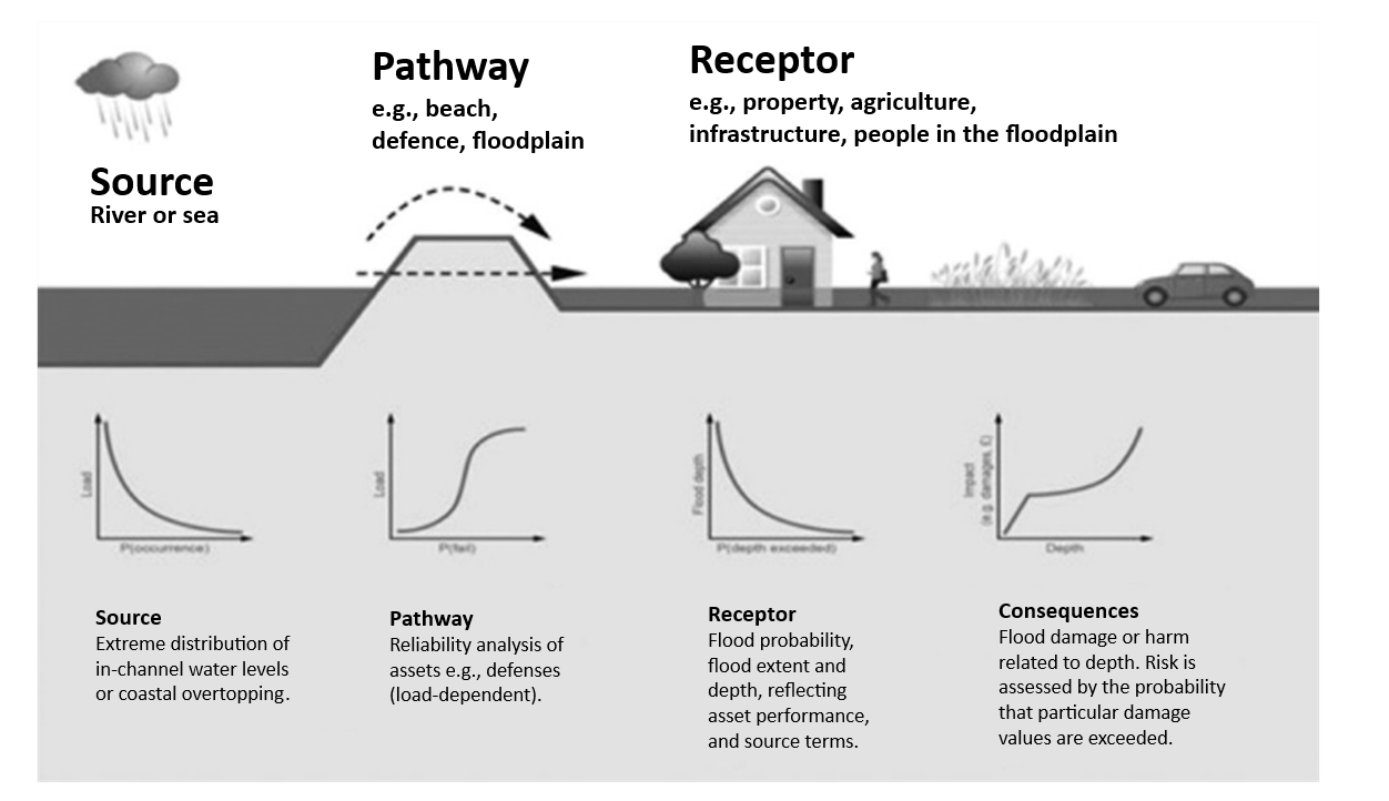
Regional analyses typically focus on understanding and characterizing flood hazard-generating sources, since it is difficult to resolve pathways and hazard interactions with receptors at large spatial scales. However, such regional analyses are typically a prerequisite for investigating pathways and hazard-receptor interactions at local (e.g., community or buildings/infrastructure) scales.

5.2.1 Hazard Sources

Sources of coastal flood hazards include elevated water levels, waves, tsunamis, and waterborne debris (including ice); which may act alone, or in combination (i.e., compound events), to generate or exacerbate flooding. Elevated river discharges, and intense precipitation are also potential sources contributing to flood hazards in coastal regions but are not addressed in this guidance. Each source can comprise multiple components; for example, coastal water levels can be elevated in response to contributions from tides, storm surges (wind and barometric set-up), sea-level rise, wave set-up, wave runup, and other factors. A preliminary assessment should consider the potential contributions or role of each source in contributing to coastal flooding, so that priorities and emphasis for more detailed analysis can be established. For example, in coastal areas situated in sheltered inlets or bays, or seas with relatively short fetches, waves may play a lesser role in driving flood hazards and may receive less attention in the analysis. In regions prone to winter sea-ice cover, the potential for attenuation of storm surges (e.g., Kim et al., 2021), tides, and waves by extensive ice cover may steer the focus of analyses to open-water season sources. As explained in Murphy et al. (2020), regional storm climatology, such as provided by Atkinson et al. (2016) for Canada’s marine coastal waters, may provide insight to storm-related drivers of coastal flooding and guide the way forward.

5.2.2 Hazard Pathways

Pathways describe how water moves through the system toward receptors, such as people, infrastructure, and valued assets. As explained by Piercy et al. (2021), understanding hazard pathways requires analysis and modelling of mechanisms leading to inundation, such as direct inundation, overtopping and breaching of coastal defences/barriers, or erosion. These pathways may guide requirements for hazard modelling. For example, static mapping of peak nearshore water levels onto digital elevation models (i.e., bathtub modelling) may be adequate in areas where direct inundation is the primary mechanism for flooding. However, such approaches may overpredict inundation in circumstances where pathways are influenced by coastal features and roughness elements, and/or can provide false evidence for the effectiveness of different flood risk management strategies during options appraisal (Piercy et al., 2021). Dynamic modelling approaches generally provide increased accuracy (Didier et al., 2019) and improved insight to flood hazard pathways, but require higher levels of effort, resources, and specialist expertise. Where flood hazards depend on the performance of flood prevention measures, the probability of flood defence failures (e.g., breaching) should be characterized, and combined with the probability of hazard source events to determine the overall probability associated with flood hazards.

5.2.3 Establishing Hazard Events and Scenarios for Analysis

Once a preliminary understanding of hazard pathways and sources is gained, a series of hazard events and scenarios is typically devised for further investigation and analysis. Hazard events may represent a single historical (hindcast) or synthetic storm event, though for risk-based analyses, a series of synthetic events with defined probabilities is usually developed. These events may be analyzed in conjunction with a variety of hazard pathway scenarios (with or without defined probabilities), multi-hazard event scenarios, planning scenarios, or flood risk management intervention scenarios, to support risk assessment and decision making. Selection of hazard events and scenarios for modelling and analysis depends on the goals/objectives and requirements of the risk assessment (Section 2.2), the timeframes relevant to decision making and adaptation, levels of uncertainty, a preliminary understanding of risk, and the outcomes of the preliminary identification and conceptualization of hazard sources and pathways described in Sections 5.2.1 and 5.2.2. For example:

• A risk assessment designed to support options appraisal for long-term flood risk management at a densely populated urban community may require more events and scenarios to be investigated than an assessment to guide planning/design for non-critical or temporary infrastructure.
• A risk assessment for a coastal community in the Salish Sea may require careful consideration of the joint probability of tide and storm surge contributions to flood hazards, whereas a community in micro-tidal regions (e.g., parts of the Beaufort Sea coast) may not be as concerned with contributions by tides.
• Risk assessments supporting planning or design for timeframes of 50 years or less may require fewer hazard scenarios than studies considering more distant time horizons, owing to the greater uncertainty surrounding climate change effects (such as sea-level rise) over longer timeframes.

The following sections provide considerations for establishing hazard events and scenarios related to two primary sources:

1. Coastal flooding driven by tides, storm surges, and waves
2. Tsunami

Although there is usually some interdependency between these sources (e.g., the tidal stage during the occurrence of a tsunami can influence the severity of tsunami-generated hazards), they are usually analyzed separately, owing to the different expertise required to analyze the hazard sources, differences in event probabilities considered, and the more specialist nature of tsunami hazard analysis.

Coastal Flood Hazard Event Probabilities

In developing coastal flood hazard events and scenarios, the preliminary assessment of the role of each source variable (i.e., tides, storm surges, waves) in contributing to coastal flooding will identify priorities and emphasis for more detailed analysis. An important part of this analysis is determining or assigning event (or response) probabilities.

A number of different methods and techniques can be used to assess the probability associated with coastal flood hazard–generating events. Statistical methods range in complexity from simple, univariate approaches that consider the likelihood of only one phenomenon (e.g., storm surge or water level) to more-complex multivariate approaches that consider the joint-probability of two or more phenomena (e.g., waves and high water levels). Establishing representative hazard events and scenarios can be challenging because there are many combinations of tides, storm surge, wave effects, and seasonal, interannual, and intradecadal factors that can combine to create severe overland flow and hazards (Murphy et al., 2020). Box 5-1 below, which paraphrases Murphy et al. (2020), summarizes four fundamentally different approaches used to assess/assign likelihoods to coastal flood hazard–generating events or hazard responses.

The choice of method for assigning hazard event or response probabilities may be driven by the requirements of a risk assessment, and the implications of this choice on the hazard and risk assessment outcomes should be considered and weighed against the complexity and resource demands for different approaches. For example, if the focus of a risk assessment is on understanding risks associated with storm surge-driven flooding at a given site, a univariate (storm surges) or bivariate (storm surges and tides) analysis may be appropriate—recognizing that this would not capture risk associated with other potential hazard sources (e.g., wave effects, debris). Similarly, response-based approaches whereby AEPs are assigned based on local flood hazard response metrics (such as depth of flooding) support, in theory, more accurate assessments of flood risk than event-based approaches (where AEPs are associated with hazard sources). However, response-based approaches are very rare, owing to the resource-intensive and complex nature of the hazard analysis. In the context of supporting decision making, which often involves comparative analyses of flood risk management measures or strategies, event-based approaches are typically adequate.

Tsunami Hazard Scenarios

If there is no anecdotal, historical, or geological evidence of past landslide-generated tsunamis in an area with generally low slopes within 5 km of the coastline in an aseismic region, it is generally not necessary to proceed with the assessment. On the other hand, areas with modest slopes and intermediate seismicity and with evidence for one or more historical events would warrant continued assessment. There is much that can be learned before failures actually occur in areas prone to underwater landslides, and hydrodynamic modelling can be used effectively to assess the tsunamigenic potential of such landslides. This recommendation is extended to subaerial failures. Landslide-generated tsunami hazard assessment should be a critical part of any infrastructure project in a moderate to high-relief coastal environment. Although definitive estimates of the frequency of occurrence and magnitude of these events are unlikely to be achieved, the analyses can place valuable constraints on the siting and design of coastal facilities.

The establishment of tsunami hazard scenarios begins with a detailed examination of historical tsunami wave heights along the coast under study. Newspaper reports from eye-witnesses and paleotsunami studies based on coastal deposits can provide a record of early historical events. Tide gauge records, from which the predicted astronomical tides have been subtracted, are the primary source of tsunami wave data during the instrumental period, although high-resolution bottom-pressure records from cabled observatory networks and DART (Detection and Recording of Tsunamis) moorings are proving increasingly valuable for more recent events. In the case of seismically generated waves on the west coast of North America, the establishment of tsunami scenarios is typically focused on major earthquakes within the widely distributed subduction zones along the “Pacific Rim of Fire”. For subaerial and subaqueous landslide-generated tsunamis, assessment considerations include the geological evidence of past failures, as well as written and oral histories of past events. Hydrodynamic modelling, combined with geological and geotechnical evidence, can be used to assess the tsunamigenic potential of landslides.

Practitioners need to work with geophysics and geotechnical experts to establish the source regions for seismically forced tsunamis. For western Canada, Gao et al. (2018) provide detailed megathrust rupture models for simulating coastal inundation from a magnitude 9.0 Cascadia Subduction Zone (CSZ) tsunami off the west coast of North America. The authors examined 15 megathrust earthquake scenarios, with emphasis on two main scenarios: a buried rupture (Model A), and a splay rupture (Model B). Although the splay-fault rupture best represents a CSZ earthquake given the present understanding of the faulting processes, both earthquake models have been used to simulate tsunamis for the southern Strait of Georgia and Boundary Bay. The National Tsunami Hazard Mapping Program of 2010 (Nicolsky et al., 2013) recommends that inundation maps from such events be computed using high tide as the initial condition for modelling. Tsunami inundation maps produced by the University of Alaska use mean higher high water (MHHW) as the initial condition (Suleimani et al., 2013), while those from Washington State use mean high water (Eungard et al., 2018). The Canadian standard of higher high water mean tide (HHWMT) is close to the U.S. standard MHHW and has been used in many tsunami-modelling projects in British Columbia (AECOM, 2013; Fine et al., 2018a, 2018b; Northwest Hydraulic Consultants Ltd., 2019). To present values of highest risk, maps of maximum tsunami wave height and current speed should be referenced to HHMWT rather than to the mean tide or to a geodetic reference.

Reconstruction of past landslide-generated tsunamis or an assessment of future risk must deal with several poorly known factors, most of which are geological or geotechnical (Bornhold & Thomson, 2012). In contrast, the hydrodynamics of landslide-generated tsunamis are now well understood due to the pioneering work of Mader (1988), Heinrich (1992), Jiang and LeBlond (1992), and others, although contributions from other processes, such as edge waves, are only now being adequately addressed (Bricker et al., 2007). A major limitation to studies of past submarine or subaerial landslides is the uncertainty regarding the volume and internal character of the landslide mass. Even if the pre- and post-failure slope morphologies are known from detailed bathymetric or topographic data, which is rarely the case, the fraction of the failed volume that generated the tsunami is generally uncertain. Commonly, the practitioner must consider a “worst-case” scenario, in which the entire mass failed at one time. Similarly, large uncertainties exist around the velocity of the failed subaerial mass as it enters the water, which is a critical factor in determining the magnitude of the resultant tsunami. Also important are the physical characteristics of the failed mass. For example, was it a single block, a highly fragmented rock mass, or did it evolve into a debris flow?

5.2.4 Hazard Model Conceptualization

A fundamental early step is to determine the questions to be answered by any models or analysis techniques being employed to quantify coastal flood hazards, and to anticipate how the models or techniques will be applied in combination with measured data to develop useful hazard information to support the risk assessment. A review and assessment of available data (Chapter 4) will inform the development of conceptual models of the system (Pye et al., 2017), and guide needs for further modelling or data acquisition.

The preferred approach to modelling depends on a variety of factors, including the anticipated exposure of the community or site to flooding from different hazard sources (e.g., considering storm climatology, topography, potential pathways), the objectives of the hazard assessment, and available data, resources, and expertise. Based on the conceptual system understanding and objectives of the modelling, an appropriate model or models can be selected. Considerations in model selection include:

• Important processes, physics, or factors affecting hazards are properly captured by the model.
• Model complexity and level of effort involved in developing, calibrating, and validating the model.
• Computational efficiency, cost, and resource demand (based on benchmarking comparisons to similar models).
• Practitioner experience with applying the model.
• Dimensionality (e.g., 2-D depth-averaged approaches are typically adequate for most tide and storm surge modelling applications, although 3-D modelling may be required under certain circumstances).
• Model has a successful track record, demonstrated by verification for relevant test cases and real-world applications.
• Required hazard metrics/outputs (Section 5.3).
• Needs for integration with mapping or GIS software.

5.3 Hazard Metrics and Indicators

Requirements to support the risk analysis will ultimately drive needs for different types of hazard metrics and indicators to be provided as output from the hazard analysis. For example, the maximum flood depth associated with a coastal storm event or scenario is most commonly used as input to vulnerability and consequence assessment. As risk analysis techniques and tools evolve, other hazard metrics relevant to assessing damages and consequences may become increasingly important or sought after (e.g., wave heights, flow velocities, duration of flooding, erosion/scour potential). Needs for hazard metrics may dictate the approach to coastal flood hazard modelling and analysis—for example, hydrodynamic modelling of overland flooding would be required to provide flow velocity output. Hazard modellers should work with those responsible for risk assessment tasks to determine the necessary model outputs and formats, and consult guidance related to risk assessment and damage estimation provided by the Federal Flood Mapping Guidelines Series (NRCan, 2021).

5.4 Modelling and Analysis Methods

The following sections provide guidance and techniques for modelling and analysis of various coastal flood hazard–generating sources and flood hazard responses, related to:

• Water levels
• Waves
• Ice and debris
• Overland flooding

5.4.1 Water Levels

Extreme high water levels are typically the primary drivers of flooding on Canada’s open coasts. Water levels in coastal regions are comprised of a variety of distinct components including mean sea level, astronomical tides, and variations in water surface elevation caused by meteorological effects (Figure 5.2). Mean water level at a given location is further impacted by relative sea-level change, which, itself, is a function of ocean thermal expansion, the contribution from diminishing glaciers and ice sheets, and vertical land motion (Greenan et al., 2018).

The tidal component of the water level is governed primarily by the gravitational forces associated with the moon and the sun (Hicks, 2006). Therefore, water level fluctuations caused by astronomical tides are generally cyclical and predictable; for example, tidal ranges fluctuate over a 14.75-day period as phasing of the principal lunar and solar semi-diurnal constituents shift (leading to spring and neap tides). The water level response at a given location caused by astronomical tides depends on a combination of the astronomical forces and shallow water effects. Meteorological phenomena, such as wind and atmospheric pressure, largely influence water levels at coastal locations and manifest in the form of wind set-up (or set-down), barometric set-up (or set-down), and wave effects (including wave set-up). The difference between the observed water level and the predicted water level, based on astronomical tides and mean sea level alone, is referred to as the water level residual. Water level residuals reflect contributions to the total water level from all sources other than astronomical tides, which may include storm surges (wind set-up/set-down and barometric set-up/set-down), and wave effects (e.g., wave set-up), seiches, or other phenomena (such as tsunami).

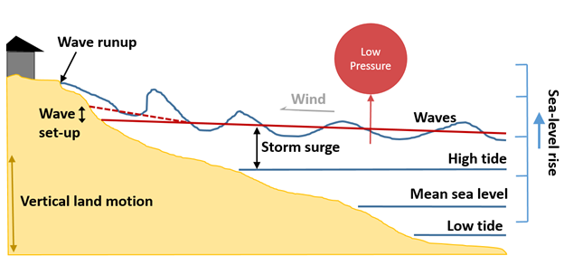
Tide Gauge Analysis

If high-quality, long-term water level measurements are available in close proximity to the risk assessment study area (i.e. sufficiently close such that the measured levels and/or fluctuations in levels reflect the characteristics of the study site), this can provide a direct basis for analyzing water level source contributions to coastal flood hazards.

Depending on the length of available water level records and the tidal range at a coastal site, it may be necessary or desirable to isolate tidal and other (e.g., meteorological) contributions to the total water level. For example, this may be important to identify extreme storm surge events in the historical record that coincided with low tides, and which, if coinciding with higher tides in the future, could result in more severe coastal flood hazards. Analysis of surge statistics from observed water level (tide gauge) measurements has been traditionally performed by computing the “residual”—the instantaneous elevation difference between the observed water level and the expected astronomic tide as predicted by harmonic analysis (Murphy et al., 2020). To estimate residuals from water level observations, one must first acquire or compute the theoretical tide at the observation location (e.g., a tide gauge) for the time period of interest. Given a time series of hourly water level observations, for example, the practitioner must compute an hourly time series of predicted tides, synchronous with the water level observations. Caution should be taken to ensure that there are no timing errors between the time series of water level observations and the predicted tides, including appropriate adjustment for time zone differences. Theoretical tides at a given location can be synthesized or predicted using principles and methods of tidal analysis and tidal prediction described by Forrester (1983). Essentially, theoretical tides are computed by summing contributions from important individual harmonic constituents at the location of interest. Constituents can be obtained by tidal harmonic analysis of water level records of sufficient length. The publicly available Institute of Ocean Sciences (IOS) Tidal Package offers a suite of programs, manuals, and test data to support tidal analysis and tidal prediction (Foreman, 2004).

Total water levels or residuals from tide gauge records may be analyzed using a variety of statistical methods and techniques (Section 5.2.3) to determine AEPs associated with extreme return levels.

Regional Tide and Storm Surge Modelling

For sites where water level data are not available, or where local flood hazards are strongly influenced by regional conditions (e.g., sea-ice conditions), regional hydrodynamic (numerical) modelling may be used to evaluate tidal and storm surge contributions to extreme water levels, assuming the model(s) can be calibrated and validated against data for nearby location(s).

General considerations for storm surge hazard analysis and modelling are provided in Box 5-4 below.

Regardless of the model’s intended purpose (e.g., to characterize regional tidal circulation and storm surges or simulate overland flood hazards), similar procedural steps apply, all of which are guided by the conceptual system definition: model selection, domain definition and discretization, initial and boundary condition prescription, parameterization of model physics, numerics, calibration, validation, and post-processing and interpretation of results. General guidance on developing and applying numerical models for simulating coastal hydrodynamics is provided in numerous documents (e.g., USACE, 2002; Pye et al., 2017; Lawless et al., 2016; Bode & Hardy, 1997; van Waveren et al., 1999; Hearn, 2008). The following list summarizes some important considerations for regional coastal hydrodynamic modelling:

• Dimensionality – Tidal circulation and storm surges are most commonly simulated using two-dimensional hydrodynamic models in which the depth-averaged shallow water equations are solved, disregarding flow variation in the vertical dimension (Dube et al., 2010; FEMA, 2016), although circumstances may exist where it is necessary to consider three-dimensional modelling (e.g., at sites with sharp vertical gradients in bathymetry or density stratification).
• Model domain/extents – When selecting the geographic domain, it is important to consider the mechanisms that drive elevated water levels associated with storm surge. For example, it may be important to choose a model domain large enough to capture atmospheric pressure and wind fields associated with synoptic-scale storm events (Dube et al., 2010; FEMA, 2016) (Figure 5.3). Nested grid models or unstructured (flexible) computational meshes can be leveraged to reduce computational demands associated with the need for both large geographic extents and high spatial resolutions in coastal areas (Dube et al., 2010; KGS, 2022).
• Topography and bathymetry representation – Accurate representation of topographic and bathymetric elevations are of crucial importance to the reliable modelling of coastal hydrodynamics. Care is therefore required when quality-checking, merging (and referencing to common datums), and integrating topography and bathymetry datasets in a numerical model.
• Spatial and temporal resolution – Spatial resolution must be high enough to capture important topographic and/or bathymetric features of relevance to simulating tidal circulation and/or storm surges and gradients in free surface elevation, but must not be so detailed that it causes impractical computational burden. Unstructured grids and nested grid techniques may be leveraged to balance these competing requirements (Dube et al., 2010; FEMA, 2016). Model time-step selection is usually driven by numerical stability requirements, but the temporal resolution of the output should be selected to capture peak water levels and durations of storm events—typically requiring output intervals of no more than 1 hour. The temporal resolution of driving input or boundary condition data (e.g., atmospheric fields) may also place practical limits on the temporal resolution of model output.
• Model forcing and boundary conditions – Surface boundary forcing for storm surge models usually consists of wind and atmospheric pressure fields, which may be derived from atmospheric models/reanalyses or parametric storm models (or both). Parameterization of air-sea momentum transfer (i.e., selection of wind drag coefficients, and the equations that describe stresses on the water surface) can have a large effect on modelled results (Dube et al., 2010), and in Arctic and Atlantic waters off Canada, may require consideration for the effects of ice (Kim et al., 2021). Selecting and applying open water boundary conditions for storm surge models is a non-trivial task (e.g., Zhai et al., 2019), and can significantly influence the storm surge response within the model domain (Dube et al., 2010). The uncertainties associated with artificial open boundary condition effects are often best mitigated by choosing large model domains with deep open water boundaries, to minimize the influence of boundary conditions on storm surges in coastal regions (Blain et al., 1994). Tidal forcing may be derived from global tide models, such as TPXO (Egbert & Erofeeva, 2002). For relatively small model domains, it may be sufficient to apply tidal forcing at offshore (open-water) boundaries, but for large domains, internal (body) forcing by tides should be applied. For nested models, boundary conditions for finer resolution grids may be supplied directly based on output from coarser resolution models.
• Model physics – Most commercially available and open-source coastal (shallow-water) hydrodynamic models incorporate the important physical processes relevant to simulating tidal circulation and storm surges in coastal regions, including: wind and atmospheric pressure forcing, tide forcing, bed friction, Coriolis forcing, wetting/drying, and turbulence.
• Model calibration and validation – The predictive skill of the numerical hydrodynamic model must be investigated through comparison with measured or observed data before it is adopted as a suitable tool for hazard and risk assessment. Calibration is an iterative process in which model parameters are adjusted until a satisfactory agreement with observational data is achieved for a given storm surge event or events. Once the practitioner is satisfied with the performance observed from the calibration process, the optimized model is tested against an independent event, or events, (not included in the calibration process) to validate model performance. Both the calibration and validation processes provide a basis to compute model skill metrics, such as root-mean-square errors in water levels, which can be presented in associated reporting materials to convey model uncertainty. Model skill metrics and variables should be assessed in the context of the objective of the hazard modelling, and acceptable uncertainty. For example, to support consequence and vulnerability assessments that rely on stage-damage curves (NRCan, 2021), it is most important to ensure high model skill at predicting peak water levels during a flood-generating event. However, other applications, such as assessing flood damages to agricultural assets and operations, may require prioritizing model skill in predicting the duration of flooding (NRCan, 2021).
• Model output – Regional hydrodynamic simulations may include long-term hindcasts, or simulations of selected extreme historical events. The output, which typically includes water levels or storm surges and flow velocities, may be used as the basis for identifying events to simulate using overland flood models (Section 5.4.4), or as direct boundary forcing for such models.

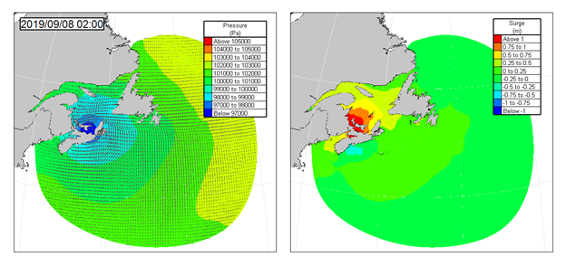
5.4.2 Waves

Waves generated by wind blowing over open water contribute to coastal flood hazards, particularly at more exposed open coast sites. Waves can contribute to hazards via:

• Wave set-up: The rise in mean water level at the shoreline, which occurs as a result of a slope in the water level required to balance the onshore flux of wave momentum (radiation stress). Wave set-up is additive to storm surges and tidal elevations, therefore potentially contributing to direct inundation or overtopping of coastal defences.
• Wave runup and overtopping: Waves impacting shorelines or coastal structures result in uprush and—if the runup elevation exceeds the crest of the beach, dune, seawall, or other shoreward features—overtopping discharges. Depending on the rate or volume of overtopping discharges and inland topography and drainage, wave overtopping discharges can contribute to flooding and failure of flood defences.
• Wave-driven sediment transport and morphodynamics: Waves are a major driver of sediment transport, which can result in changes to nearshore bathymetry and shore topography, over a variety of timescales. For example, breaching of sandy dunes during storm events can lead to overtopping discharges and direct inundation of landward areas. Shoreline erosion (including scour) and recession over various timescales can undermine coastal defences, or increase exposure to waves and extreme water levels, leading to increased flood hazards.
• Wave forces and impacts: Direct exposure to wave action can result in significant dynamic loads, exacerbating flood hazards.
• Wave-driven currents: Longshore currents, undertow, and rip currents generated by waves can exacerbate flood hazards in exposed open coast areas.
• Wave-transported debris: Storm waves can mobilize and transport objects in coastal zones, such as ice, trees and tree fragments, logs, and human-caused debris (plastics, etc.), which can then directly impact buildings and other receptors, or create jams/accumulations that lead to backwater effects or diversion of floodwaters.

Answers to the following questions may be used to guide the definition of wave hazard scenarios:

• Potentially, how exposed is the community or site to wind waves (considering the orientation of the shoreline relative to offshore waves; wave generation potential on local fetches; potential source-receptor pathways, such as erosion or overtopping; nearshore topography and bathymetry influences on wave transformation processes; range of water levels)?
• Are there correlations or dependencies between wave-related hazards and other factors contributing to coastal flood hazards (e.g., storm surges, tides) at this location?

Wave Data Analysis

Evaluation of wave contributions to coastal hazards generally requires an understanding of offshore (open water) wave conditions, including swell and wind-sea contributions, wave propagation and transformation processes in nearshore areas, and wave interactions with shore-based features and structures (e.g., FEMA, 2019). Techniques with varying levels of complexity may be applied to characterize waves at a particular location, depending on a variety of factors, including the level of anticipated risk, the availability of field or modelled data, the importance of waves in contributing to the overall flood hazard, and the goals/objectives of the hazard assessment. Guidance on selecting appropriate types of analysis is provided by Murphy et al. (2020), and is summarized in Box 5-5 below.

Wave Modelling

Preliminary analyses to develop a conceptual understanding of processes contributing to coastal flood hazards at a given site should help determine the potential role and contribution of wave effects, and therefore, modelling needs. These needs may range from application of basic empirical formulae to estimate sea states based on wind speeds, wind durations, and/or fetch lengths (e.g., CIRIA et al., 2007), to more sophisticated numerical modelling involving transformation of waves as they propagate from offshore to nearshore and/or overland.

Offshore wave conditions (sea state spectra or spectral parameters) may be derived from gridded (model-based) metocean products (such as reanalyses), wave buoy records (see Wave Data Analysis under Section 5.4.2) or calculated based on empirical formulae using wind data as input. The latter should typically be restricted to preliminary analyses or fetch-limited seas, where gridded data may be unavailable or unreliable.

Depending on the definition of extreme events (including joint occurrence of waves and other processes contributing to coastal flood hazards) and scenarios informing the risk assessment, a variety of approaches may be taken to transform offshore waves to the nearshore, for example (in decreasing order of computational cost):

• Long-term, dynamical transformation of offshore waves to nearshore (e.g., multi-decadal hindcast).
• Transformation of a matrix of selected offshore wave conditions to the nearshore, which is then used to reconstruct a long-term nearshore wave climate using the offshore time series as input (e.g., Cornett & Zhang, 2008).
• Transformation of selected offshore wave events (e.g., extreme wave conditions with specified annual exceedance probabilities) to the nearshore (e.g., Murphy et al., 2019).

Local conditions may determine requirements for the analysis. For example, depending on nearshore water depths, waves may be depth-limited (i.e., nearshore wave heights are constrained by shallow water depths, which induce breaking). This means that the range of nearshore wave conditions can essentially be decoupled from offshore conditions, potentially simplifying nearshore wave transformation modelling requirements. Wave set-up, surf beat, and other non-linear processes can still necessitate detailed analysis. As with any numerical modelling of coastal processes, model calibration and validation (e.g., using local wave measurements from buoys or other sources, wave run-up elevation or debris line surveys, or other sources), ideally capturing storm conditions, is critically important.

The output parameters from wave transformation modelling (e.g., Figure 5.4) may include nearshore wave heights, periods, directions, wave spectra, and changes to mean water levels (set-up and set-down). Additionally, wave-current interaction modelling can determine the effects of currents (tidal, fluvial, or wind-driven) on wave conditions, as well as the effects of wave conditions on nearshore currents. Physical modelling can also be used to evaluate wave transformations and wave-current interactions, generally over small scales (up to a few kilometres), but at typically greater cost than numerical modelling.

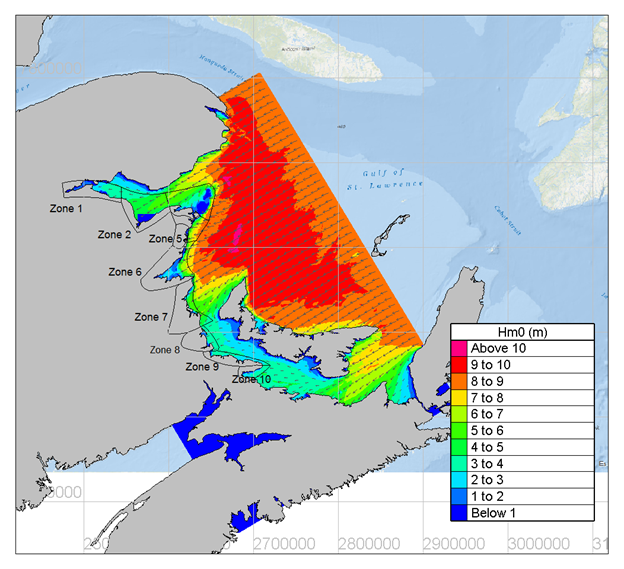
Different types of models and approaches are required to evaluate surf-zone processes, wave set-up, runup, and overtopping of coastal features and defences, and/or wave-structure interactions. Depending on the application and required output to characterize flood hazards, approaches may include the use of empirical formulae to calculate wave runup elevations on shorelines (e.g. KGS, 2022) or mean overtopping discharges (for input to overland flood models) (EurOtop, 2018), sophisticated phase-resolving numerical wave models, or physical (laboratory) models (Figure 5.5). Guidance on these topics is provided in Murphy et al. (2020).

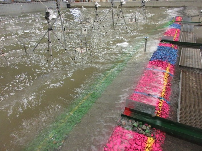
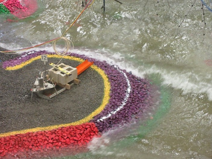
The required outputs from wave modelling will depend on the needs to inform the risk assessment, and the role of waves in contributing to coastal flood hazards. For example, a simple approach to consider wave contributions may involve mapping wave run-up elevations to assess whether or not buildings, infrastructure or valued assets will be exposed to wave effects, or whether coastal defences are overtopped by waves. In areas where wave overtopping discharges contribute to overland flooding and inundation, but communities and valued assets are not directly exposed to incident waves, water depth and/or flow velocity output from overland flood models and depth-damage curves may be sufficient to assess risk. For buildings and infrastructure on exposed open coasts where direct wave action can contribute to damage, wave heights and periods may be used in combination with fragility functions that utilize those inputs. In some circumstances, more sophisticated wave-structure interaction modelling may even be required to assess damages (e.g., wave impacts on critical infrastructure types for which fragility functions do not exist).

5.4.3 Ice and Debris

Canada’s Atlantic and Arctic coasts are prone to seasonal ice cover. Depending on conditions, ice can either reduce, contribute to, or exacerbate coastal flood hazards. Shorefast ice and large regions of continuous (or near-continuous) ice cover acts as a barrier at the ocean surface, preventing or limiting momentum transfer from winds to the sea surface, and therefore reducing the potential for large waves and storm surges. Ice cover can effectively reduce open-water fetch distances, suppressing wave generation, and attenuate waves and storm surges (Shapiro & Simpson, 1953; Squire, 2007; Manson et al., 2016a; Kim et al., 2021). However, intermediate ice concentrations and mobile ice floes can actually enhance air-sea momentum transfer through increased surface roughness from drag, potentially amplifying storm surges (Birnbaum & Lüpkes, 2002). Furthermore, mobile ice can pose hazards when onshore winds cause ice pile-up and ride-up (Barker & Timco, 2017; Kovacs & Sodhi, 1980; Forbes & Taylor, 1994; Forbes et al., 2004, 2018). Climate change impacts, such as sea-ice retreat, can result in increased wave heights in fetch-limited seas (Casas-Prat et al., 2018) and result in longer open-water seasons that are more conducive to coastal flood hazards. The potential for ice to affect or interact with coastal flood hazards should be considered by reviewing available historical data and projected future changes in ice conditions. The decline in sea-ice cover and lengthening of open-water seasons observed in Canada’s Arctic and Atlantic shelf seas in recent decades is projected to continue in the 21st century, and will likely result in increased exposure to waves and storm surges in these regions (Greenan et al., 2018). Traditionally, coastal flood hazards in ice-affected seas were typically evaluated for open-water season only, based on the assumption that the most extreme events always coincide with open-water conditions. However, flood-generating storm surge events are known to occur during periods of extensive ice cover (Ferguson et al., 2022), and relatively straightforward ice parameterizations are increasingly being applied in hydrodynamic (Joyce et al., 2019; Kim et al., 2021) and spectral wave models (Liu et al., 2020) to capture the influence on storm surges and waves. Advances in, and application of, these types of models is likely to be increasingly important in the context of climate change effects on ice conditions and seasonality of ice cover.

Similar to mobile ice floes, large quantities of waterborne debris, whether from natural sources (e.g., uprooted trees or sea wrack) or human-caused sources (e.g., manufactured timber, escaped logs from logging activities, shipping containers, boats, fragments of damaged buildings or infrastructure) can contribute to damage during flooding or tsunami events (Murphy et al., 2021). In particular, tsunamis can result in mobilization of debris over large distances inland (Leonard & Bednarski, 2014; Nistor et al., 2017). Methods for evaluating waterborne debris impact loads on structures and loads resulting from damming or accumulation of debris are provided by FEMA (2011) and ASCE (2016), which depend on the size and weight of the debris. However, the extent to which debris hazards can presently be included in risk-based analyses is constrained by the lack of fragility functions for consequence analysis, limited knowledge of debris characteristics in different regions, and the lack of predictive modelling capability to describe debris transport on the coast (Murphy et al., 2021).

5.4.4 Overland Flood Inundation

Overland flood hazard modelling typically involves combining information about nearshore hazard sources (e.g., water levels and wave conditions from the analyses described in Sections 5.4.1 through 5.4.3) with known pathways (e.g., wave overtopping, direct inundation) to identify flood-affected areas (inundation extents) and generate flood hazard metrics (e.g., water depths, velocities, etc.). This is normally a separate modelling exercise from the regional analyses described in Sections 5.4.1 through 5.4.3, although nested and unstructured grid techniques may allow for integration of regional and local numerical hydrodynamic models.

Static versus Dynamic Modelling Methods

Modelling of overland flooding may involve 1) application of process-based (hydrodynamic) numerical models or simply 2) involve mapping representative floodwater elevations onto digital elevation models (DEMs), referred to as “bathtub” modelling. The latter approach does not take into account the dynamics of floodwater propagation or pathways to flooding, and typically only provides information about inundation/water depths (i.e., not velocities, wave action, flood durations, or other hazard metrics). However, the lower complexity and fewer resources required to implement bathtub modelling can make it an attractive approach, depending on the complexity of topography in flooded areas, pathways to flooding, the importance of local process dynamics, and hazard metrics required to support the risk assessment.

Passive, bathtub modelling approaches may also enable mapping of flood depths at a higher resolution than hydrodynamic modelling by circumventing the need for interpolation or resampling to lower resolution computational meshes (Didier et al., 2019).

Some hydrodynamic models now utilize a hybrid approach, whereby modelled parameters (e.g., water depths, velocities, etc.) output from a coarser resolution computational mesh are mapped back to raw, high resolution DEMs. Another hybridization of process-based modelling and static water level mapping involves “hydro-enforcement” of DEMs (e.g., manipulation of elevations to represent discrete flow paths, such as culverts, bridge openings, etc.) prior to propagating water elevations landward (Webster et al., 2004; Poppenga et al., 2014). The potential for non-process-based or static mapping techniques to grossly mischaracterize the hazard risk (e.g., Barnard et al., 2019) should be considered prior to pursuing such approaches. A comparison of bathtub modelling and hydrodynamic modelling conducted for a case study on the Atlantic coast shows reasonable agreement between the methods in predicting inundation extents (Figure 5.6).

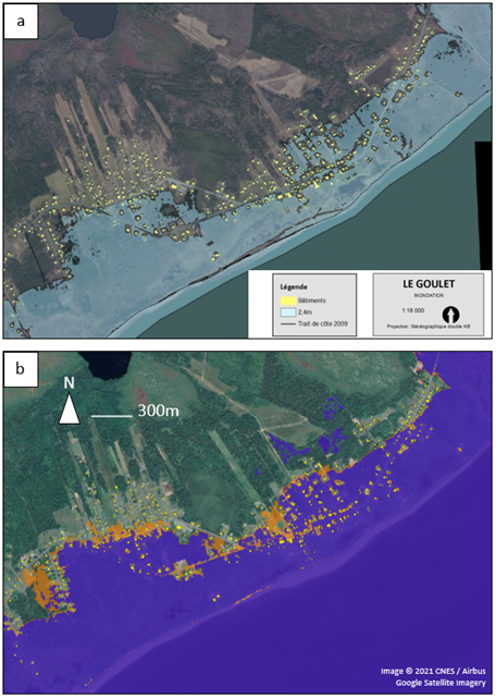
Representation of Infrastructure in Flood Hazard Areas

In developed areas, infrastructure such as buildings, walls, roads, and flood defences can obstruct floodwaters creating complex preferential flow pathways with implications on flood propagation, wave propagation and flow velocity (National Research Council, 2009). Similarly, drainage infrastructure (e.g., culverts) can hydraulically connect land parcels that would otherwise be disconnected below certain flood stages. When developing overland flood models, practitioners should gain some knowledge of the physical landscape (e.g., cliffs versus sloped beach) and constructed features (e.g., roads, dikes, seawalls, culverts, causeways) affecting flood propagation in the study area. For example, linear features such as dikes, road embankments, or culverts may have a significant impact on flood propagation and distribution and may require careful attention to ensure proper representation in model computational meshes/grids (see Box 5-7 below).

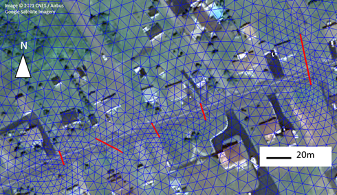
Depending on the scale of the hazard assessment and the level of detail required, practitioners may need to incorporate the impacts of buildings, infrastructure, and flood defences into the flood modelling and analyses. Drainage infrastructure, such as culverts and ditches can be incorporated into elevation datasets (and, by extension, flood modelling) via hydro-enforcement, or incorporated in two-dimensional hydrodynamic models as sub-grid scale features/structures. Hydro-enforced DEMs include special adjustment of elevations to reflect hydraulic and hydrologic connectivity (Poppenga et al., 2014). There are a number of methods to simulate flow obstruction caused by buildings and elevated structures in flood models. Schubert & Sanders (2012) describe four methods to incorporate impacts of buildings, varying in complexity and required effort. Some methods (such as the “building-resistance” method) described by Schubert & Sanders (2012) aim to simulate the flow resistance or drag exerted by the buildings without explicitly resolving the exact geometry or footprint of the buildings. Other methods (such as the “building-hole” method) integrate individual building footprints into the model domain, permitting fine-detail simulation of preferential flow pathways between buildings. One of the key considerations is that the building-resistance method allows the building footprints to store water, while the building-hole approach does not. This consideration is often more relevant for river and creek flooding than for coastal flooding, but there may still be situations where onshore storage effects will need to be considered for coastal floods. The level of detail in which infrastructure (including drainage infrastructure) can be incorporated into flood modelling is limited, in part, by the resolution and the quality of the elevation and infrastructure data available. Practitioners should consider spatial thresholds for flow-structure interaction. For example, do the objectives of the analysis warrant simulation of building-scale flow-structure interaction? Or perhaps generalizations can be applied to simulate flow-structure interaction at the neighbourhood scale. Schubert & Sanders (2012) discuss the implications of several different approaches on predictive skill and computational effort.

Overland Flood Hazard Hydrodynamic Modelling Considerations

If applying hydrodynamic models for overland flood hazard simulation, many of the considerations described in the Regional Tide and Storm Surge Modelling section under Section 5.4.1 also apply:

• Dimensionality – Two-dimensional (depth-averaged) models are almost always adequate for overland flooding applications.
• Model domain/extents – The model should extend sufficiently far inland to exceed the reach and elevation of the most severe floods being simulated. This may require trial and error or conservative assumptions based on regional analyses.
• Topography and bathymetry representation – Accurate representation of topographic and bathymetric elevations are of crucial importance to the reliable modelling of overland flooding. Care is therefore required when quality-checking, merging (and referencing to common datums), and integrating topography and bathymetry datasets in a numerical model. Particular care should be given to linear features, such as culverts, road embankments, and dikes.
• Spatial and temporal resolution – Spatial resolution must be high enough to capture important topographic and/or bathymetric features of relevance to simulating overland flooding and to capture flow pathways. This may require sensitivity testing to identify the coarsest resolution that can be adopted without compromising accuracy. This will usually involve consideration of the Courant-Friedrichs-Lewy criterion. Model time-step selection is usually driven by numerical stability requirements, but the temporal resolution of the output should be selected to capture peak water levels and durations of storm events.
• Model forcing and boundary conditions – Offshore/nearshore boundary conditions are typically derived from regional models or analysis. For example, water levels (or water levels and velocities) from regional analyses may be applied at the offshore boundary of the overland flooding model. In cases where direct inundation does not occur, boundary conditions for the overland flooding model may consist of mean overtopping discharges from wave modelling or empirical calculations. Bed friction parameter selection is typically a key focus for model calibration and validation and may be informed by land classifications derived from satellite imagery, lidar, or other remote-sensing techniques. If necessary, model boundary conditions may include flow contributions from rivers and upland drainage.
• Model physics – Most commercially available and open-source two-dimensional (shallow-water) hydrodynamic models incorporate the important physical processes relevant to simulating overland flooding.
• Model calibration and validation – Sourcing data for overland flood model calibration is often a significant challenge. Ideally, during- and post-flood high water mark survey data will be available for historically significant flood events, but is often lacking. High-resolution satellite imagery during severe flood events can also be used to support overland flood model calibration by enabling identification of areas inundated by water, but often misses the peak of a short-term flooding event or is obscured by cloud cover. Debris/wrack line surveys or observations, photographic evidence, or descriptive stories obtained from those present during flood events can also be used for semi-quantitative or qualitative assessment of model skill (see Box 4-3 in Section 4.3). Individuals or communities may also often have private written or photographic documentation. Tapping this “citizen science” can be a key resource. These data may be used to supplement quantitative data sources to develop a more expansive basis for model skill assessment.
• Model output – Typically, this is driven by requirements to support the risk analysis, and may include inundated areas, water depths, and flow velocities. Consequences and damages are generally quantified based on the number and types of assets exposed to floodwaters, as well as the depth of flooding (NRCan, 2021). Therefore, desired model outputs may include maximum flood extents and flood depths produced by the storm surge event. Alternatively, practitioners may be requested to provide information regarding the temporal variation of the floodwaters during the storm surge event to inform the investigation of flood propagation or flooding duration. Some risk assessment procedures use joint depth-velocity metrics to evaluate human safety/stability (Cox et al., 2010; Jonkman & Penning-Rowsell, 2008) and damage to infrastructure (FEMA, n.d.; NRCan, 2021). When preparing model outputs (peak or time series), practitioners should discard results calculated during the model spin-up period preceding model stability.

5.5 Tsunami Hazard Modelling

5.5.1 Model Development

Tsunami wave generation, propagation and inundation are most commonly modelled using the 2D shallow-water equations (SWE) and non-hydrostatic models. In tsunami models, vertical particle acceleration is neglected and the horizontal components of velocity are uniform with depth. Because the horizontal wave length of tsunamis is much larger than the water depth scale, these assumptions are usually correct for seismically generated tsunamis. The non-linear shallow-water equations can be derived in a number of different ways, but all fundamentally arise from an integration of the Euler or Navier-Stokes equations with the assumption of vertically invariant horizontal velocity and hydrostatic pressure. Due to their simple and well-studied nature, the shallow-water equations can be solved by a wide variety of numerical schemes, such as the finite difference, finite volume, and finite element approaches.

TUNAMI, COMCOT, MOST, and GeoClaw are popular packages (based on SWE) in the tsunami modelling field, which have been validated successfully through benchmarks and water level records from historical tsunami events. MOST (Method Of Splitting Tsunami) was originally developed by researchers at the University of Southern California (Titov & Synolakis, 1998); COMCOT (Cornell Multi-grid Coupled Tsunami Model) was developed at Cornell University (Liu et al., 1994); and TUNAMI (Tohoku University’s Numerical Analysis Model for Investigation), was developed in Japan (Imamura et al., 1988). All three models solve the same depth integrated and 2D horizontal (2DH) non-linear shallow-water equations with different finite difference algorithms. The GeoClaw software (LeVeque et al., 2011) is a computing package under constant development that solves the SWE based on high-resolution shock capturing finite volume methods and incorporates an adaptive mesh refinement (AMR) technique for multi-scale tsunami modelling and has been validated against various tsunami benchmarks (Gonzalez et al., 2011).

The SWE models, by definition, lack the capability of simulating dispersive waves, which could be dominating features in landslide-generated tsunamis (Lynett & Liu, 2002) and can be important for far-field tsunamis travelling a long distance. To address this issue, a different set of governing equations must be employed. In this regard, Boussinesq-type models, which represent an extension to SWEs, are used as they can better describe the wave dispersions, e.g., Kirby et al. (1998) and Wei et al. (1995) developed a fully non-linear Bossinesq wave model known as FUNWAVE-TVD and COULWAVE (Cornell University Long and Intermediate Wave Model, Lynett et al., 2002). The FUNWAVE model employs a hybrid finite-volume and finite-difference MUSCL-TVD scheme and is formulated in both Cartesian and spherical coordinates with Coriolis effects for application to ocean basin-scale problems. Another non-hydrostatic approach, with the same order of approximation, but different from Boussinesq model formalism, was developed by Yamazakiet al. (2010). The software, named NEOWAVE (Non-hydrostatic Evolution of Ocean WAVEs), was used for seismic- and landslide-generated tsunami modelling. Similar software, named NHWAVE (Non-Hydrostatic Wave Model), based on a different numerical approach, was developed at the University of Delaware (Ma et al., 2012). Although non-linear non-hydrostatic models can simulate more complete physics associated with wave dispersion, they are computationally more demanding. The advantage of SWE models is that they need less computational effort compared to other models and the simulated results for seismic-generated tsunamis are reliable. As a consequence, SWE models are more commonly used for full lifespan tsunami simulations.

5.5.2 Nested Grid Formulation

Accurate numerical simulation of tsunami waves in rapidly shoaling coastal regions requires setting up the model domain as a series of grids of ever finer spatial and temporal resolution. The use of nested grids makes it possible to resolve tsunami wave configurations as they propagate into increasingly shoaling coastal regions. The use of nested grids for numerical modelling has several principal requirements:

1. Grid cell sizes are obtained by dividing the initial, large-scale coarse numerical grid by an integer, typically 3 to 5. Integers larger than this can lead to grid interface problems.
2. Nested grids are needed in near-coastal areas and the coarse “parent” grid should be of sufficient extent to resolve possible feedback effects that the nested grid may have on the parent grid during the simulation time.
3. A good interface between the inner and outer domains is required to avoid errors and model instability associated with point matching between the different grids. This should allow two-way fluxes without trapping shorter waves at the inner domain boundaries.
4. High-resolution bathymetry, external forcing, and observations are needed for model domain set-up, initialization, and validation at each domain level.

5.5.3 Domain and Grid Resolution

In order to simulate the wave propagation from the tsunami source in deep ocean and predict the inundation in coastal areas of interest, multiple grids must be designed in the nesting approach. The choice of model grids takes into account the need for high spatial resolution to accurately resolve the reflection and transformation of the waves and the need for a large spatial extent to capture the full source area.

To resolve significant features that impact inundation, the computational grid should be fine enough that the feature covers more than three cells. The computational grid domain should have enough extent to capture important tsunami wave dynamics. While topographic grid resolution is controlled by the available data sources, the numerical grid resolution is controlled by the wavelengths that need to be properly resolved. Generally, for a reasonable numerical representation of the waveform, there should be at least 10 grid points covered in a single wavelength. In practice, this can be challenging due to the changing length of the wave through shoaling and non-linear generation of shorter waves in shallow water. In practice, a horizontal grid spacing of 10 m is adequate for proper resolution of detailed tsunami evolution for a site-specific coastal and onshore inundation modelling application, while a 40–60 m resolution is likely sufficient for runup estimation and regional hazard assessments. In the deep ocean, grid lengths of a few kilometers may provide proper resolution.

5.5.4 Numerical Convergence

Numerical convergence, a test to demonstrate that the hydrodynamic predictions of interest are not dependent on the grid resolution, should be performed. A reasonable approach is to increase/decrease the target resolution by 25% and compare the results. Here, the target resolution is the resolution of expected convergence, for example 10 m for a detailed, coastal/onshore simulation. If the output of interest is the maximum water surface elevation near a particular location, these values as predicted by the simulations with different resolutions should be presented and compared. If the results are within a reasonable tolerance, for example, 5% of the target resolution result, it can be stated that the target resolution is convergent. Earlier tsunami hazard assessment work performed with FUNWAVE-TVD along the U.S. East Coast (e.g., Grilli et al., 2015; Schambach et al., 2018) indicated that convergence required coastal grid with at least 30-m resolution. Preferably, 10 m should be used for tsunami inundation/runup results to converge, which is also the recommendation of the U.S. NTHMP. More recently, in order to assess convergence for coastal hazard assessment along the French Riviera, Nemati et al. (2019) performed a newer set of simulations and concluded that tsunami runup obtained using 40-m and 10-m resolution grids appear to be mutually consistent, indicating that convergence of these simulations may have been achieved.

5.5.5 Time Steps

The numerical scheme in most tsunami models is explicit, and the maximum permissible time step for stability is determined by the Courant-Friedrichs-Lewy (CFL) criterion (Courant et al., 1967) and is therefore connected to the grid size used. With this condition, the Courant number, which describes the number of grid cells crossed by a water particle during a simulation time step (Ata, 2018), must be a positive value and smaller than one (0<C≤1); C=0.5 is usually recommended for simulations, and represents a trade-off between model stability, model accuracy, and computational demand. In general, the finer the grid resolution, the smaller the time steps, in order to maintain model stability. Smaller time steps make the model more computationally expensive.

5.5.6 Model Reference Level

Model simulations are generally conducted for tsunami arrival times that coincide with times of Canadian Vertical Datum of higher high water mean tide (HHWMT). The National Tsunami Hazard Mapping Program of 2010 (Nikolsky et al., 2013) recommends that inundation maps be computed using high tide as the initial condition for modelling. Alaska University uses mean higher high water (MHHW) as the initial condition (Suleimani et al., 2013), while Washington State inundation maps are created using mean high water for initial conditions (Eungard et al., 2018). The Canadian standard HHWMT is close to the U.S. standard MHHW and has been used for many tsunami modelling projects in coastal British Columbia for Victoria (AECOM, 2013), for Seal Cove and Victoria Cove (Fine et al., 2018a, 2018b), and for Prince Rupert (Northwest Hydraulic Consultants Ltd., 2019). Accordingly, to present values of highest risk, maps of maximum tsunami wave height and current speed are referenced to HHMWT, rather than to the mean tide or to a geodetic reference.

5.5.7 Model Validation and Verification

As recommended by the National Tsunami Hazard Mitigation Program (NTHMP, 2011) it is necessary that all numerical models used in inundation mapping be validated and verified. The term “validation” refers to confirming that the model results are reasonably consistent with available data. Verification, on the other hand, refers to confirming that a model is free of errors. Validation is best done by subjecting each model to a series of benchmark tests commonly accepted by the community. The three usual categories of reference data used for defining benchmark tests for tsunami numerical model validation are: (i) analytical solutions; (ii) laboratory experiments; and (iii) field measurements. The verification of numerical models is a continuous process. Even proven numerical models must be subjected to additional testing as new knowledge/methods or better data are obtained. New benchmark tests must also be defined to address new tsunami source characteristics or complex coastal impact. Therefore, all existing numerical models, according to their capability, must be tested regularly against a selected set of benchmark tests, for validation and verification. The official suite of benchmark tests was originally assembled based on the recommendations of Synolakis et al. (2007).

For real world cases, where possible, the simulated wave heights, wave arrival time, and the general wave trend should match well with the observed time series at available tide gauges, pressure gauges, and other observations of the event. Then, the maximum computed runup should be compared with the field observations, where available. The evaluation of model results versus the observations should be supported with statistical methods, for example, by calculating the mean and standard deviation, and root-mean-square-difference parameters.

5.5.8 Initial Condition

Successful simulation of tsunami propagation and accurate prediction of the arrival time and wave height at different locations rely on a correct estimate of the earthquake fault plane geometry and fault type. Interplate faults in subduction zones are responsible for most of the large historical tsunamis. For such ruptures, the resulting seafloor displacement can be estimated using linear elastic dislocation theory (Okada, 1985).

The vertical displacement of the seafloor (uplift and subsidence) due to an earthquake is defined as the initial condition. Based on the assumptions that the upward seafloor deformation is impulsive, and seawater is incompressible, the initial ocean free surface profile mimics the deformation. This assumption is acceptable for seismic-generated tsunamis since the rupture time is much shorter than the wave period. For a given source-region condition specified by either the initial free surface elevations or a time history of seafloor displacement, hydrodynamic models can accurately simulate propagation of a tsunami over a long distance, provided that accurate bathymetric data exists for the propagation path.

Note that the deformation due to an earthquake should also be added into the digital elevation model (DEM). This is important when these changes extend toward the land (topography). For example, for a Cascadia Subduction Zone scenario, some parts of the west coast of Vancouver Island will sink after the earthquake due to subsidence, which must be taken into account for tsunami inundation modelling.

5.5.9 Boundary Condition

There are three main types of boundary conditions: open, solid-wall, and absorbing boundaries. For open boundary conditions, the flow variables from the inner boundary cell are copied to the ghost cell to allow zero gradients at the boundary; the conditions can also be prescribed to impose inflow and outflow conditions. For closed boundary conditions, the normal velocity and the gradient in water depth are set to zero at solid boundaries. For example, Giles et al. (2020) describe the application of ghost cells to prescribe boundary conditions.

In FUNWAVE, a wall boundary condition and an absorbing boundary condition are implemented following Kirby et al. (1998). The boundary condition for the first outer nested grid is an absorbing (“sponge”) boundary. The length of the sponge layer is usually taken to be one or two times a typical tsunami wavelength.

5.5.10 Model Runtime

Model runtime should be sufficient to capture the maximum inundation of the tsunami simulation and to estimate a time period when hazardous waves are present. The selection of runtime mainly depends on the distance between the tsunami source region and the inundation area being studied. For example, for a study of inundation of the Boundary Bay in British Columbia region from an Alaska 1964-type earthquake, 15 hours of simulation was adopted, while for a Cascadia Subduction Zone earthquake, 10 hours was chosen. For a crust-fault scenario, which is located near to Boundary Bay, it was found that 3 hours of simulation time is sufficient to model the key features of tsunami waves from generation to inundation on the coast.

5.5.11 Friction

Although bed friction is relatively unimportant for tsunami propagation in the deep ocean, energy dissipation by bottom friction plays a major role in deterring the maximum wave runup at the coast. On a fundamental level, frictional dissipation is caused by interaction of the wave motions with the seafloor. A smooth, sandy beach may generate minor dissipation, while a coral reef or a mangrove forest will have a greater role in reducing tsunami energy (Fernando et al., 2005).

Friction is modelled using the Manning term, which consists of a quadratic function characterized by a bottom friction coefficient. A bottom “Manning n” friction coefficient that best represents the overall terrain roughness should be used. If the Manning coefficient is not prescribed, a typical constant value of n= 0.025 s/m^1/3, which represents a sandy bed, can be used for the whole tsunami modelling domain. However, if the material of the bed is known, then the friction factor that best approximates the variable landscape terrain should be used for inundation modelling.

5.5.12 Model Stability

In order to deal with numerical instability, some adjustments may be needed. A rapidly varying bathymetry may cause numerical noise due to a large gradient in the source term and an unreasonably large bottom slope may cause numerical instability. Based on past experience with FUNWAVE, depth gradients in the model greater than 1.0 should be avoided.

Wetting and drying interfaces are another possible source of numerical instability. Using very small values of minimum depth may cause a large velocity at a wetting-drying point, resulting in a small time step. Adjusting the minimum depth may help if an instability occurs. A minimum depth of 0.1 m is considered a default value of the wetting-drying threshold for the highest-resolution (10 m) grid. For lower-resolution grids, a greater minimum depth could be selected. As an example, for the Boundary Bay project, ONC used 0.1 m and 0.3 m as minimum depths for the 10-m and 30-m resolution grids, respectively.

For tsunami simulations, bed friction can be an important factor for the flow in the inundation zone and for runup estimations, although the inclusion of the friction may affect the numerical stability near the wet-dry front when the water depth vanishes. In this regard, a minimum water depth of 0.1 m for the field-scale modelling is suggested.

The FUNWAVE model uses a Froude number cap to avoid an unrealistic flow velocity in extremely shallow water. Unrealistic flow velocities usually occur at wetting-drying interfaces. The default value for the Froude cap is 10.0. Using a smaller value, such as 3.0 or smaller, can avoid the problem and improve the model efficiency in terms of the CFL algorithm. That said, a Froude cap smaller than 1.5 is not suggested because it may cap velocities of the leading edge of a flooding current.

5.5.13 Output

Numerical simulations provide a suite of outputs that can be presented in different ways. These model outputs should support the requirements for risk assessment tasks. The outputs from a tsunami model must include water surface elevation, tsunami-induced currents (as east-west and north-south components), the inundation extent, maximum tsunami wave height, maximum tsunami-induced currents and could include a hazard rating (such as depth x velocity). The output interval time should be reasonable enough to show the progressive changes of these parameters. The output interval should be at least every five minutes, although smaller intervals (e.g., every one minute) are preferable.

For tsunami hazard analysis, the typical output types should be presented as following.

Snapshots of surface elevation and current speed

Snapshots of water surface elevation or velocity illustrate the parameter in two or three spatial dimensions at a specific time. A series of snapshots from the open ocean to near coastal areas is useful in graphically displaying the spatial evolution of the tsunami in a technical report.

Time series of model output

Time series are used to present the temporal variations in a simulated parameter at a single location. These diagrams are useful for presenting ocean surface elevation time histories near a site or at some offshore location, for example, the location at the offshore limit of the high-resolution coastal inundation grid. The temporal resolution of time series should be sufficient to delineate the peaks, troughs, and wave period.

Maps of tsunami maxima

Maps of maximum tsunami wave height, flood extent, and tsunami-induced currents provide important graphic displays of a specific simulation. These images are useful for showing the maximum levels reached near a particular location.

Tabulated results

In addition to the graphical products, a hazard analysis should also include a summary table of the site-specific results. Such a table should include tsunami properties for each site, such as: initial tsunami arrival time, peak wave arrival time, maximum and minimum wave amplitudes, dominant wave periods, and maximum tsunami-induced currents. These properties should be listed for all tsunami sources included in the site-specific analysis, for all relevant locations at the site.

5.6 Climate Change Effects

Climate change is, and is expected to continue, influencing coastal flood hazards in several ways:

• Relative sea-level change will alter the frequency and severity of flooding driven by tides, storm surges, and wave effects.
• In coastal regions prone to seasonal ice cover, retreating sea ice and longer open-water seasons will likely lead to increased frequency and severity of coastal flooding.
• The frequency and intensity of storms may change in the future, resulting in changes in the frequency and severity of storm surge and wave contributions to coastal flood hazards.

The following sections provide some guidance on incorporating some of these effects in various aspects of hazard modelling and analysis.

5.6.1 Relative Sea-Level Change

Relative sea-level projections (James et al., 2021) are provided by the Canadian Centre for Climate Services at climatedata.ca (direct link (https://climatedata.ca/variable/, scroll to sea-level change), based on the Fifth Assessment Report of the Intergovernmental Panel on Climate Change (Church et al., 2013) (see Chapter 6 for a description of climate scenarios and relative sea-level variability across Canada). Sea-level projections provide the foundational information upon which to incorporate other information on storm surge, high tides, and waves, to ascertain future high-water levels and flooding hazard.

The sea-level projections are available on climatedata.ca every decade to the year 2100. Depending on project scope and timeframe, the practitioner may wish to consider sea-level projections one or two decades in the future, or projections at century-end. At many localities, and for many applications, the projected sea-level rise corresponding to the 95th percentile of the high-emissions RCP8.5 scenario may be of the greatest interest, as it provides the largest amount of projected relative sea-level rise. For practitioners with low tolerance to the risks of sea-level rise, it may also be appropriate to consider the high-end scenario at 2100, which assumes an additional 65 cm of global sea-level rise, based on assumed rapid evacuation of portions of the Antarctic Ice Sheet, added to the median projection of RCP8.5. This scenario corresponds to 139 cm of sea-level rise at 2100. Even higher scenarios at 2100 (up to 2.5 m) are provided by the U.S. National Oceanic and Atmospheric Administration (Sweet et al., 2017). The practitioner may wish to consider these larger values if tolerance to risk of sea-level rise is extremely low or if a longer timeframe, extending toward 2200, is being considered.

In regions where sea level is projected to fall, such as Hudson Bay and much of the Canadian Arctic Archipelago (see Chapter 4), navigation hazards arising from reduced depth-under-keel may be of interest. In this case, the 5th percentile of the low-emissions RCP2.6 would provide the largest projections of relative sea-level fall for consideration. This projection would also be relevant for potential stranding of coastal infrastructure or valued natural features, such as approaches and beaches used for sea-lift.

The climatedata.ca website provides maps of projected relative sea-level change. Tables of projected relative sea-level change can be downloaded for specified locations. Practitioners carrying out regional investigations, spanning distances of many kilometres or more, may wish to utilize national geospatial files of projected sea-level change (James et al., 2021). These projected values can be combined in a number of ways with waves, storm surge, and tidal variations to discern future flooding hazards. As research evolves, models should consider the effects of land uplift or subsidence from earthquakes on future sea level projections. At this time, however, guidance cannot be provided as to how to incorporate these effects.

For example, the Canadian Extreme Water Level Adaptation Tool (CAN-EWLAT) is a science-based planning tool for climate change adaptation of coastal infrastructure related to future water-level extremes and changes in wave climate (https://www.bio.gc.ca/science/data-donnees/can-ewlat/index-en.php). The tool includes two main components: 1) vertical allowance and 2) wave climate. CAN-EWLAT was developed primarily for Fisheries and Oceans Canada (DFO) Small Craft Harbours (SCH) locations, but it can be applied by coastal planners dealing with infrastructure along Canada’s ocean coastlines. Vertical allowances are recommended changes in the elevation of coastal infrastructure required to maintain the current level of flooding risk in a future scenario of sea-level rise. Past extreme water-level events recorded on tide gauges are combined in a rigorous statistical manner with projected relative sea-level change to provide the sea-level allowances.

Other approaches vary in complexity. Hydrodynamic modelling of present-day flooding levels due to storm surge, tidal variations, and waves can provide the extent and depth of present-day flooding. Under a scenario of future sea-level rise, the flood depths can be increased accordingly to estimate future flood depths. A more physically realistic approach would involve dynamic simulation of flooding by adjusting model bathymetry or mean water level assuming a specified amount of relative sea-level rise (see Box 5-12 below). This would capture the physics of water flow and would provide a better estimate of future flooding conditions. Future changes to infrastructure, including changes to coastal barriers, such as dikes, would need to be explicitly incorporated into digital elevation models if their effects on future flooding levels are to be accurately ascertained. Simulating geomorphology changes over the long time-scales relevant to sea-level rise effects is impractical, particularly considering uncertainty surrounding driving physical forces (e.g., wave climate), but in many regions, it is likely an important factor affecting how sea-level rise will affect coastal flood hazards. Where relevant, consideration should be given to exploring alternative geomorphic responses or outcomes to better understand associated risks.

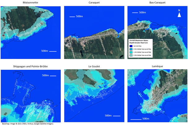
5.6.2 Changes in Ice Conditions

The decline in sea-ice cover and lengthening of open-water seasons observed in Canada’s coastal regions in the last half-century is projected to continue in the 21^st century and will likely result in increased exposure to waves and storm surges (Greenan et al., 2018). The state of knowledge surrounding projected changes in sea-ice conditions is summarized by Greenan et al. (2018). Hydrodynamic models incorporating the physics of air-ice-water interactions may be used to explore scenarios, sensitivities, and potential impacts of changing ice cover on storm surges and tides (Kim et al., 2021).

5.6.3 Changes in Storm Surges, Waves, and Climate Variability

There is generally low confidence in projected changes in waves and storm surges in Canada’s coastal regions, except in regions with seasonal ice cover (Greenan et al., 2018). Climate cycles, such as El Niño-La Niña Southern Oscillation (ENSO) can cause water levels in the northeast Pacific to fluctuate by +0.12/-0.04 m on average (Barnard et al., 2015). Since projections surrounding the future frequency and intensity of ENSO events are uncertain (Barnard et al., 2015), it may be prudent to consider future flood hazards under peak El Niño conditions. Downscaled projections of future extreme storm surges and waves are beginning to emerge for some Canadian coastlines (Casas-Prat et al., 2018; Casas-Prat & Wang, 2019). However, the robustness of projections, particularly in seas where ice is not a controlling factor, is challenged by inherent uncertainties in driving atmospheric circulation-related parameter projections from climate models (Shepherd, 2014; Casas-Prat et al., 2018). If robust projections of changes to storm behavior (intensity, direction of storm tracks, duration), storm surges, and extreme waves become available, this information could be incorporated into coastal flood hazard modelling and analysis to determine future hazards. Until such time as robust projections are available, sensitivity analyses and/or scenario-based testing is advisable.

5.7 References

AECOM. (2013). Modelling of Potential Tsunami Inundation Limits and Run-Up (Project No. 6024 2933).

American Society of Civil Engineers. (2017). Minimum Design Loads and Associated Criteria for Buildings and Other Structures (7-16). American Society of Civil Engineers.

Ata, R. (2018). Telemac2d User Manual (Version v8p0).

Atkinson, D. E., Forbes, D. L., & James, T. S. (2016). Chapter 2: Dynamic coasts in a changing climate. In Lemmen, D.S., Warren, F.J., James, T.S. & Mercer Clarke, C.S.L. (Eds.). Canada’s Marine Coasts in a Changing Climate (27-68). Government of Canada.

Barker, A. and Timco, G. W. (2017). Maximum pile-up heights for grounded ice rubble. Cold Regions Science and Technology, 135, 62-75.

Barnard, P. L., van Ormondt, M., Erikson, L. H., Eshleman, J., Hapke, C., Ruggiero, P., Adams, P. N. & Foxgrover, A. C. (2014). Development of the Coastal Storm Modeling System (CoSMoS) for predicting the impact of storms on high-energy, active-margin coasts. Natural Hazards, 74(2), 1095-1125.

Barnard, P. L., Short, A. D., Harley, M. D., Splinter, K. D., Vitousek, S., Turner, I. L., Allan, J., Banno, M., Bryan, K. R., Doria, A. & Hansen, J. E. (2015). Coastal vulnerability across the Pacific dominated by El Niño/Southern Oscillation. Nature Geoscience, 8(10), 801-807.

Barnard, P. L., Erikson, L. H., Foxgrover, A. C., Hart, J. A. F., Limber, P., O’Neill, A. C., Van Ormondt, M., Vitousek, S., Wood, N., Hayden, M. K., & Jones, J. M. (2019). Dynamic flood modeling essential to assess the coastal impacts of climate change. Scientific Reports, 9(1), 4309. https://doi.org/10.1038/s41598-019-40742-z

Bastidas, L. A., Knighton, J. & Kline, S. W. (2016). Parameter sensitivity and uncertainty analysis for a storm surge and wave model. Natural Hazards and Earth System Sciences, 16(10), 2195-2210.

Benoit, M., Marcos, F., & Becq, F. (1996). Development of a third-generation shallow-water wave model with unstructured spatial meshing. Proc. International Conference on Coastal Engineering, 465-478.

Bernardara, P., Mazas, F., Kergadallan, X., & Hamm, L. (2014). A two-step framework for over-threshold modelling of environmental extremes. Natural Hazards and Earth System Sciences, 14, 635–647. https://doi.org/10.5194/nhess-14-635-2014

Bernier, N. B., & Thompson, K. R. (2006). Predicting the frequency of storm surges and extreme sea levels in the northwest Atlantic. Journal of Geophysical Research, 111. https://doi.org/10.1029/2005JC003168

Bernier, N. B., Thompson, K. R., Ou, J., & Ritchie, H. (2007). Mapping the return periods of extreme sea levels: allowing for short sea level records, seasonality, and climate change. Global and Planetary Change, 57, 139-150, https://doi.org/10.1016/j.gloplacha.2006.11.027

Birnbaum, G., & Lüpkes, C. (2002). A new parameterization of surface drag in the marginal sea ice zone. Tellus A: Dynamic Meteorology and Oceanography, 54(1), 107–123. https://doi.org/10.3402/tellusa.v54i1.12121

Blain, C. A., Westerink, J. J. & Luettich Jr, R. A. (1994). The influence of domain size on the response characteristics of a hurricane storm surge model. Journal of Geophysical Research: Oceans, 99(C9), 18467-18479.

Bode, L. & Hardy, T. A. (1997). Progress and recent developments in storm surge modeling. Journal of Hydraulic Engineering, 123(4), 315-331.

Bornhold, B. D. & Thomson, R. E. (2012). Chapter 10: Tsunami hazard assessment related to slope. In Clague, J. J. & Douglas, S. (Eds.), Landslides: Types, Mechanisms and Modeling. Cambridge University Press.

Bricker, J. D., Munger, S., Pequignet, C., Wells, J. R., Pawlak, G. & Cheung, K. F. (2007). ADCP observations of edge waves off Oahu in the wake of the November 2006 Kuril Islands tsunami. Geophysical Research Letters, 34(23).

Casas-Prat, M., Wang, X. L., & Swart, N. (2018). CMIP5-based global wave climate projections including the entire Arctic Ocean. Ocean Modelling, 123, 66–85. https://doi.org/10.1016/j.ocemod.2017.12.003

Casas-Prat, M., & Wang, X. L. (2020). Projections of extreme ocean waves in the Arctic and potential implications for coastal inundation and erosion. Journal of Geophysical Research: Oceans, 125(8). https:/doi.org/10.1029/2019JC015745

Caston, M. (2021). Tsunamigenic Potential of Crustal Faults in the Southern Strait of Georgia and Boundary Bay. [Master’s thesis, University of Victoria]. http://hdl.handle.net/1828/13351

Church, J.A., Clark, P. U., Cazenave, A., Gregory, J. M., Jevrejeva, S., Levermann, A., Merrifield, M. A., Milne, G. A., Nerem, R. S., Nunn, P. D., Payne, A. J., Pfeffer, W. T., Stammer, D., & Unnikrishnan, A. S.. (2013). Sea Level Change. In Stocker, T.F., D. Qin, G.-K. Plattner, M. Tignor, S.K. Allen, J. Boschung, A. Nauels, Y. Xia, V. Bex & P.M. Midgley (Eds.), Climate Change 2013: The Physical Science Basis. Contribution of Working Group I to the Fifth Assessment Report of the Intergovernmental Panel on Climate Change. Cambridge University Press.

CIRIA, CUR, & CETMEF. (2007). The Rock Manual. The use of rock in hydraulic engineering (2nd edition). CIRIA.

Cornett, A. & Zhang, J. (2008). Nearshore wave energy resources, Western Vancouver Island, BC (Technical Report CHC-TR-51). Canadian Hydraulics Centre. https://www.nrcan.gc.ca/sites/www.nrcan.gc.ca/files/canmetenergy/files/pubs/CHC-TR-051.pdf

Couasnon, A., Sebastian, A., & Morales-Nápoles, O. (2018). A Copula-based Bayesian network for modeling compound flood hazard from riverine and coastal interactions at the catchment scale: An application to the Houston ship channel, Texas. Water, 10(9), 1-19.

Courant, R., Friedrichs, F. & Lewy, H. (1967). On the Partial Difference Equations of Mathematical Physics. IBM Journal of Research and Development, 11(2), 215-234.

Cox, R. J., Shand, T. D., & Blacka, M. J. (2010). Australian Rainfall and Runoff Revision Project 10: Appropriate Safety Criteria for People—Stage 1 Report (P10/S1/006). Engineers Australia.

Daigle, R. (2017). Updated Sea-Level Rise and Flooding Estimates for New Brunswick Coastal Sections Based on IPCC 5th Assessment Report. R.J. Daigle Enviro.

de Vries, H., Breton, M., de Mulder, T., Krestinitis, Y., Ozer, J., Proctor, R., Ruddick, K., Salomon, J.C. & Voorips, A. (1995). A comparison of 2D storm surge models applied to three shallow European seas. Environmental Software, 10(1), 23-42. https://doi.org/10.1016/0266-9838(95)00003-4

DHI. (2017). Mike 21 SW Scientific Documentation. https://manuals.mikepoweredbydhi.help/2017/Coast_and_Sea/M21SW_Scientific_Doc.pdf

Didier, D., Baudry, J., Bernatchez, P., Dumont, D., Sadegh, M., Bismuth, E., Bandet, M., Dugas, S., & Sévigny, C. (2019). Multihazard simulation for coastal flood mapping: Bathtub versus numerical modelling in an open estuary, Eastern Canada. Journal of Flood Risk Management, 12. https://doi.org/10.1111/jfr3.12505

Dube, S. K., Murty, T. S., Feyen, J. C., Cabrera, R., Harper, B. A., Bales, J. D., & Amer, S. (2010). Storm Surge Modeling and Applications in Coastal Areas. In Chan, J. C. L. & Kepert, J. D. (Eds.), Global Perspectives on Tropical Cyclones: From Science to Mitigation, World Scientific Publishing.

Egbert, G. D., & Erofeeva, S. Y. (2002). Efficient Inverse Modeling of Barotropic Ocean Tides. Journal of Atmospheric and Ocean Technology, 19, 183–204.

Eungard, D. W., Forson C., Walsh T. J., Gica E, & Arcas, D. (2018). Tsunami Hazard maps of the Anacortes-Bellingham area, Washington – model results from a ~2500-year Cascadia Subduction Zone earthquake scenario. Washington Geological Survey, Map series 2018-2, June 2018.

Federal Emergency Management Agency. (n.d.). Multi-hazard Loss Estimation Methodology: Flood Model—Hazus-MH Technical Manual. Department of Homeland Security.

Federal Emergency Management Agency. (2011). Coastal Construction Manual (FEMA P-55 / Volume II).

Federal Emergency Management Agency. (2016). Guidance for Flood Risk Analysis and Mapping: Coastal Water Levels.

Federal Emergency Management Agency. (2019). Guidance for Flood Risk Analysis and Mapping: Determination of Wave Characteristics.

Ferguson, S., Provan, M., Murphy, E., & Kim, J. (2022). Numerical Simulation of Coastal Flood Hazard in the Acadian Peninsula Region of New Brunswick (NRC-OCRE-2021-TR-060). National Research Council Canada.

Fernando, H. J. S., McCulley, J. L., Mendis, S. G., & Perera, K. (2005). Coral poaching worsens tsunami destruction in Sri Lanka. Eos Trans. AGU, 86(33) 301-304. https://doi.org/10.1029/2005EO330002

Fine, I. V., Thomson, R. E., Lupton, L. M., & Mundschutz, S. (2018a). Numerical modelling of an Alaska 1964-type Tsunami at the Canadian Coast Guard Base in Seal Cove, Prince Rupert, British Columbia. Tech. Rep. Hydrogr. Ocean Sci. 321: v+ 33p.

Fine, I. V., Thomson, R. E., Lupton, L. M., & Mundschutz, S. (2018b). Numerical modelling of a Cascadia subduction zone tsunami at the Canadian Coast Guard base in Seal Cove, Prince Rupert, British Columbia (Canadian Technical Report of Hydrography and Ocean Sciences 321). Fisheries and Oceans Canada.

Forbes, D. L. & Taylor, R. B. (1994). Ice in the shore zone and the geomorphology of cold coasts. Progress in Physical Geography: Earth and Environment, 18, 59-89. https://doi.org/10.1177/030913339401800104

Forbes, D. L., Parkes, G. S., Manson, G. K., & Ketch, L. A. (2004). Storms and shoreline retreat in the southern Gulf of St. Lawrence. Marine Geology, 210(1-4), 69-204.

Forbes, D. L., Bell, T., Manson, G. K., Couture, N. J., Cowan, B., Deering, R. L., Hatcher, S. V., Misiuk, B., & St-Hilaire-Gravel, D. (2018). Coastal environments and drivers. In Bell, T. and Brown, T.M. (Eds.). From Science to Policy in the Eastern Canadian Arctic: An Integrated Regional Impact Study (IRIS) of Climate Change and Modernization (210-249). ArcticNet. http://www.arcticnet.ulaval.ca/pdf/media/29170_IRIS_East_full%20report_web.pdf

Foreman, M. G. G. (2004). Manual for tidal heights analysis and prediction (Pacific Marine Science Report 77-10). Institute of Ocean Sciences.

Forrester, W. D. (1983). Canadian Tidal Manual. Department of Fisheries and Oceans, Canadian Hydrographic Service.

Gao, D., Wang, K., Insua, T. L., Sypus, M., Riedel, M., & Sun, T. (2018). Defining megathrust tsunami source scenarios for northernmost Cascadia. Natural Hazards, 94, 445–469. https://doi.org/10.1007/s11069-018-3397-6

Giles, D., Kashdan, E., Salmanidou, D. M., Guillas, S., & Dias, F. (2020). Performance analysis of Volna-OP2–massively parallel code for tsunami modelling. Computers & Fluids, 209, 104649.

González, F. I., LeVeque, R. J., Chamberlain, P., Hirai, B., Varkovitzky, J. and George, D. L. (2011). Validation of the GeoClaw Model. GeoClaw Tsunami Modeling Group, University of Washington.

Greenan, B. J. W., James, T. S., Loder, J. W., Pepin, P., Azetsu-Scott, K., Ianson, D., Hamme, R. C., Gilbert, D., Tremblay, J.-E., Wang, X. L., & Perrie, W. (2018). Chapter 7: Changes in oceans surrounding Canada. In Bush, E. & Lemmen, D.S. (Eds.), Canada’s Changing Climate Report (pp. 343–423). Government of Canada. https://changingclimate.ca/CCCR2019/

Greene, H. G., Barrie, J. V., & Todd, B.J. (2018). The Skipjack Island fault zone: An active transcurrent structure within the upper plate of the Cascadia subduction complex. Sedimentary Geology, 378, 61-79.

Grilli, S. T., O’Reilly, C., Harris, J. C., TajalliBakhsh, T., Tehranirad, B., Banihashemi, S., Kirby, J. T., Baxter, C. D. P., Eggeling, T., Ma, G., & Shi, F. (2015) Modeling of SMF tsunami hazard along the upper US East Coast: detailed impact around Ocean City, MD. Natural Hazards 76(2), 705–746. https://doi.org/10.1007/s11069-014-1522-8

Haigh, I., Wadey, M., Wahl, T., Ozsoy, O., Nicholls, R., Brown, J., Horsburgh, K., & Bouldby, B. (2016). Spatial and temporal analysis of extreme sea level and storm surge events around the coastline of the UK. Scientific Data, 3, 160107. https://doi.org/10.1038/sdata.2016.107

Hawkes, P. J. (2008). Joint probability analysis for estimation of extremes. Journal of Hydraulic Research, 46(S2), 246-256.

Hearn, C. J. (2008). The Dynamics of Coastal Models. Cambridge University Press.

Heinrich, P. (1992). Nonlinear water waves generated by submarine and aerial landslides. Journal of Waterway, Port, Coastal, and Ocean Engineering, 118(3), 249-266.

Hicks, S. D. (2006). Understanding Tides. National Oceanic and Atmospheric Administration.

Horsburgh, K. J. & Wilson, C. (2007). Tide‐surge interaction and its role in the distribution of surge residuals in the North Sea. Journal of Geophysical Research: Oceans, 112, C08003.

H. R. Wallingford. (1998). The Joint Probability of Waves and Water Levels: JOIN-SEA. A rigorous but practical new approach (Report SR 537). Lancaster University.

Imamura, F., Shuto, N., & Goto, C. (1988). Numerical simulations of the transoceanic propagation of tsunamis. [Conference proceedings]. 6th Congress Asian and Pacific Regional Division, IAHR, Japan.

Irish, J.L., Resio, D.T., & Divoky, D. (2011). Statistical properties of hurricane surge along a coast. Journal of Geophysical Research: Oceans, 116(C10).

James, T. S., Robin, C., Henton, J. A., & Craymer, M. (2021). Relative Sea-level Projections for Canada based on the IPCC Fifth Asssessment Report and the NAD83v70VG National Crustal Velocity Model (Open File 8764). Ressources naturelles Canada. https://doi.org/10.4095/327878

Jane, R. A., Simmonds, D. J., Gouldby, B. P., Simm, J. D., Dalla Valle, L., & Raby, A. C. (2018). Exploring the potential for multivariate fragility representations to alter flood risk estimates. Risk Analysis, 38(9), 1847-1870.

Jiang, L. & LeBlond, P. H. (1992). The coupling of a submarine slide and the surface waves which it generates. Journal of Geophysical Research: Oceans, 97(C8), 12731-12744.

Jonkman, S. N., & Penning-Rowsell, E. (2008). Human instability in flood flows. Journal of the American Water Resources Association, 44. https://doi.org/10.1111/j.1752-1688.2008.00217.x

Joyce, B. R., Pringle, W. J., Wirasaet, D., Westerink, J. J., Van der Westhuysen, A. J., Grumbine, R., & Feyen, J. (2019). High-resolution modeling of western Alaskan tides and storm surge under varying sea ice conditions. Ocean Modelling, 141, 101421. https://doi.org/10.1016/j.ocemod.2019.101421

Kelsey, H. M., Sherrod, B. L., Blakely, R. J., & Haugerud, R. A. (2012). Holocene faulting in the Bellingham forearc basin: Upper‐plate deformation at the northern end of the Cascadia subduction zone. Journal of Geophysical Research: Solid Earth, 117(B3).

KGS (2022) Climate Change Flood Risk Mapping Study for Placentia, Carbonear, Victoria and Salmon Cove (21-3217-002).

Kim, J., Murphy, E., Nistor, I., Ferguson, S., & Provan, M. (2021). Numerical Analysis of Storm Surges on Canada’s Western Arctic Coastline. Journal of Marine Science and Engineering, 9(3), 326. https://doi.org/10.3390/jmse9030326

Kim, J., Murphy, E., Ferguson, S., Provan, M., & Nistor, I. (2024). Numerical simulation of storm surges in the Beaufort Sea and coastal flood hazards in the Hamlet of Tuktoyaktuk, Northwest Territories (NRC-OCRE-2022-TR-015). National Research Council Canada.

Kirby, J., Wei, G., Chen, Q., Kennedy, A., & Dalrymple, R. (1998). FUNWAVE 1.0, fully nonlinear Boussinesq wave model documentation and users manual (Tech. Rep. Research Report No. CACR-98-06). Center for Applied Coastal Research, University of Delaware.

Kovacs, A. and Sodhi, D. S. (1980). Shore ice pile-up and ride-up: Field observations, models, theoretical analyses. Cold Regions Science and Technology, 2, 210-288.

Lawless, M., Hird, M., Rodger, D., Gouldby, B., Tozer, N., Pullen, T., Saulter, A. & Horsburgh, K. (2016). Investigating coastal flood forecasting — Good practice framework (Report SC140007). Environment Agency (United-Kingdom). https://assets.publishing.service.gov.uk/media/60362b4a8fa8f5480bbb4545/Coastal_flood_forecasting___a_good_practice_framework_-_report.pdf

Leonard, L. J. & Bednarski, J. M. (2014). Field survey following the 28 October 2012 Haida Gwaii tsunami. Pure and Applied Geophysics, 171(12), 3467-3482.

LeVeque, R. J., George, D. L., & Berger, M. J. (2011). Tsunami modeling with adaptively refined finite volume methods. Acta Numerica, 20, 211-289. https://doi.org/10.1017/S0962492911000043

Lin, L., Demirbilek, Z., Mase, H., Zheng, J., & Yamada, F. (2008). CMS-Wave: A Nearshore Spectral Wave Processes Model for Coastal Inlets and Navigation Projects (ERDC/CHL TR-08-13). US Army Corps of Engineers, Coastal and Hydraulics Laboratory.

Liu, D., Tsarau, A., Guan, C. & Shen, H.H. (2020). Comparison of ice and wind-wave modules in WAVEWATCH III^® in the Barents Sea. Cold Regions Science and Technology, 172, 103008.

Liu, J. C., Lence, B. J., & Isaacson, M. (2010). Direct Joint Probability Method for Estimating Extreme Sea Levels. Journal of Waterway Port Coastal and Ocean Engineering, 136(1), 66-76.

Liu, P. L.-F., Cho, Y.-S., Yoon, S. B., & Seo, S. N. (1995). Numerical simulations of the 1960 Chilean tsunami propagation and inundation at Hilo, Hawaii. In Tsuchiya, Y. & Shuto, N. (Eds.), Tsunami: Progress in Prediction. Disaster Prevention and Warning (99-115). Springer Dordrecht.

Lynett, P. & Liu, P. L.-F. (2002). A numerical study of submarine-landslide-generated waves and run-up. Proceedings of the Royal Society of London A, 458(2028), 2885–2910. https://doi.org/10.1098/rspa.2002.0973

Lynett P., Wu T.-R., Liu P. L.-F. (2002). Modeling wave runup with depth-integrated equations. Coastal Engineering 46(2), 89–107.

Ma, G., Shi, F., & Kirby, J. T. (2012). Shock-capturing non-hydrostatic model for fully dispersive surface wave processes. Ocean Modelling, 43–44, 22-35.

Mader, C. L. (1988). Numerical Modeling of Water Waves, University of California Press.

Manson, G. K., Davidson-Arnott, R. G. D., & Ollerhead, J. (2016a). Attenuation of wave energy by nearshore sea ice: Prince Edward Island, Canada. Journal of Coastal Research, 32(2), 253-263. https://doi.org/10.2112/JCOASTRES-D-14-00207.1

Manson, G. K., Davidson-Arnott, R. G. D., & Forbes, D. L. (2016b). Modelled nearshore sediment transport in open-water conditions, central North Shore of Prince Edward Island, Canada. Canadian Journal of Earth Sciences, 53(1), 101-118. https://doi.org/10.1139/cjes-2015-0090

Masina, M., Lamberti, A., & Archetti, R. (2015). Coastal flooding: A copula based approach for estimating the joint probability of water levels and waves. Coastal Engineering, 97, 37-52.

Mazas, F. & Hamm, L. (2016). An event-based approach for extreme joint probabilities of waves and sea levels. Coastal Engineering Proceedings, 1(35), 20.

Mazas, F. & Hamm, L. (2017). An event-based approach for extreme joint probabilities of waves and sea levels. Coastal Engineering, 122, 44-59.

Ministry of Forests, Lands, Natural Resource Operations and Rural Development. (2018). Flood Hazard Area Land Use Management Guidelines. Ministry of Water, Land and Air Protection, Province of British Columbia. https://www2.gov.bc.ca/assets/gov/environment/air-land-water/water/integrated-flood-hazard-mgmt/flood_hazard_area_land_use_guidelines_2017.pdf

Muis, S., Verlaan, M., Winsemius, H. C., Aerts, J. C., & Ward, P. J. (2016). A global reanalysis of storm surges and extreme sea levels. Nature Communications, 7.

Murphy, E. & Khaliq, M. N. (2017). Input to Canadian national guideline for flood hazard mapping: Coasts & lakes (OCRE-TR-2017-005). National Research Council Canada.

Murphy, E., Lyle, T., Wiebe, J., Hund, S. V., Davies, M., & Williamson, D. (2020). Coastal Flood Risk Assessment Guidelines for Building and Infrastructure Design Applications (CRBCPI-Y5-R2). National Research Council Canada.

Murphy, E., Osborne, P., & Clohan, D. (2016). Water level and tsunami design criteria for LNG marine terminals in BC. [Conference proceedings] 14th Triennial International Ports Conference, American Society of Civil Engineers, New Orleans.

Murphy, E., Pilechi, A., & Cousineau, J. (2018). Regional wave run-up study for the province of New Brunswick. Technical Report (OCRE-TR-2018-026). National Research Council of Canada. Ocean, Coastal and River Engineering.

Murphy, E., Boisvert, J., McLean, R., Pilechi, V., Cousineau, J., Sushama, L., & Liang, Z. (2019). Wave run-up contributions to coastal flood hazards in New Brunswick. [Proceedings]. Annual Conference: Canadian Society for Civil Engineering 2019, Fredericton.

Murphy, E., Nistor, I., Cornett, A., Wilson, J., & Pilechi, A. (2021). Fate and transport of coastal driftwood: A critical review. Marine Pollution Bulletin, 170, 112649.

Narayan, S., Hanson, S., Nicholls, R. J., Clarke, D., Willems, P., Ntegeka, V., & Monbaliu, J. (2012). A holistic model for coastal flooding using system diagrams and the Source–Pathway–Receptor (SPR) concept. Natural Hazards and Earth System Science, 12(5), 1431-1439.

National Research Council. (2009). Mapping the Zone: Improving Flood Map Accuracy. The National Press.

National Tsunami Hazard Mitigation Program (NTHMP). (2011). Proceedings and Results of Model Benchmarking Workshop, NOAA Special Report.

Nemati F., Grilli S. T., Ioualalen M., Boschetti L., Larroque C., & Trevisan J. (2019). High resolution coastal hazard assessment along the French Riviera from co seismic tsunamis generated in the Ligurian fault system. Natural Hazards, 96, 553-586. https://doi.org/10.1007/s11069-018-3555-x

Nicolsky, D. J., Suleimani, E. N., Haeussler, P. J., Ryan, H. F., Koehler, R. D., Combellick, R. A., & Hansen, R. A. (2013). Tsunami inundation maps of Port Valdez, Alaska (Report of Investigation RI 2013-1). Alaska Division of Geological Geophysical Surveys.

Nistor, I., Goseberg, N., & Stolle, J. (2017). Tsunami-driven debris motion and loads: A critical review. Frontiers in Built Environment, 3, 2.

Northwest Hydraulic Consultants Ltd. (2019). The City of Prince Rupert Tsunami Flood Risk Assessment (Final report). City of Prince Rupert. https://www.princerupert.ca/sites/7/files/2023-06/20190621%203003349%20Prince%20Rupert%20Tsunami%20Report.pdf

Natural Resources Canada. (2021). Federal Flood Damage Estimation Guidelines for Buildings and Infrastructure (Version 1.0, General Information Product 124e).

Okada Y. (1985). Surface deformation due to shear and tensile faults in a half-space. Bulletin of the Seismological Society of America, 75, 1135–1154.

Ontario Ministry of Natural Resources. (2001). Great Lakes – St. Lawrence River System and Large Inland Lakes Technical Guide for Flooding, Erosion and Dynamic Beaches [computer file] Watershed Science Centre, ISBN 0-9688196-1-3.

Piercy, C. D., Simm, J. D., Bridges, T. S., Hettiarachchi, M., & Lodder, Q. (2021). Chapter 5: NNBF Performance. In Bridges, T. S., King, J. K., Simm, J.D., Beck, M. W., Collins, G., Lodder, Q. & Mohan R.K. (Eds.), International Guidelines on Natural and Nature-Based Features for Flood Risk Management. U.S. Army Engineer Research and Development Center.

Poppenga, S. K., Worstell, B. B., Danielson, J. J., Brock, J., Evans, G. A., & Heidemann, H. K. (2014). Hydrologic enforcement of lidar DEMs. U.S. Geological Survey.

Pugh, D. T., & Vassie, J. M. (1980). Applications of the joint probability method for extreme sea level computations. Proceedings of the Institution of Civil Engineers, 69, 959–975. https://doi.org/10.1680/iicep.1980.2179

Pugh, D. T. (1987). Tides, Surges and Mean Sea-Level. John Wiley & Sons Ltd. ISBN 0 471 91505 X.

Pye, K., Blott, S.J., & Brown, J. (2017). Advice to Inform Development of Guidance on Marine, Coastal and Estuarine Physical Processes Numerical Modelling Assessments. NRW Report No: 208, 139 pp, Natural Resources Wales, Cardiff.

Reeve, D., Horillo-Caraballo, J., Fox, A., Simmonds, D., Kwan, S., Pan, S., & Greaves, D. (2012). Coastal defence evaluation: An SPRC approach. Proc. 33rd Int. Conf. on Coastal Eng., Santander.

Resio, D. T., Asher, T. G., & Irish, J. L. (2017). The effects of natural structure on estimated tropical cyclone surge extremes. Natural Hazards, 88, 1609–1637. https://doi.org/10.1007/s11069-017-2935-y

Resio, D.T., Irish, J., & Cialone, M. (2009). A surge response function approach to coastal hazard assessment-part 1: basic concepts. Natural Hazards, 51(1), pp.163-182.

Resio, D. T. & Westerink, J. J. (2008). Modeling the physics of storm surges. Physics Today, 61(9).

Sanchez, A., Li, H., Brown, M., Rosati, J., Demirbilek, Z., Wu, W., & Reed, C. (2014). Coastal Modelling System: Mathematical Formulations and Numerical Methods. U.S. Army Corps Of Engineers, Coastal Inlets Research Program ERDC/CHL TR-14-2, Vicksburg.

Schambach L., Grilli S. T., Kirby J. T., & Shi F. (2018). Landslide tsunami hazard along the upper US East Coast: effects of slide rheology, bottom friction, and frequency dispersion. Pure Appl Geophys. https://doi.org/10.1007/s00024-018-1978-7

Schubert, J. E., & Sanders, B. F. (2012). Building treatments for urban flood inundation models and implications for predictive skill and modeling efficiency. Advances in Water Resources, 41, 49–64. https://doi.org/10.1016/j.advwatres.2012.02.012

Shapiro, A., & Simpson, L. (1953). The effect of a broken ice field on water waves. Eos Transactions of the American Geophysical Union, 34, 36–42.

Squire, V. A. (2007). Of ocean waves and sea-ice revisited. Cold Regions Science and Technology, 49(2), 110–133. https://doi.org/10.1016/j.coldregions.2007.04.007

Suleimani, E. N., Nicolsky, D. J., & Koehler, R.D. (2013). Tsunami Inundation Maps of Sitka, Alaska. Report of Investigations 2013-3, State of Alaska, Department of Natural Resources, Division of Geological and Geophysical Surveys, Fairbanks, AK, 76 p., 1 sheet, scale 1:250,000. https://doi.org/10.14509/26671

Sweet, W., Kopp, R., Weaver, C., Obeysekera, J., Horton, R., Thieler, E., & Zervas, C. (2017). Global and Regional Sea Level Rise Scenarios for the United States. NOAA.

Synolakis C. E., Bernard E. N., Titov V. V., Kanoglu, U., & González, F.I. (2007). OAR PMEL-135 Standards, criteria, and procedures for NOAA evaluation of tsunami numerical models. Technical report, NOAA Tech. Memo. OAR PMEL-135, NOAA/Pacific Marine Environmental Laboratory, Seattle, WA.

The SWAN Team. (2009). SWAN User Manual. Delft University of Technology, Delft.

Titov, V. V. and Synolakis, C. E. (1998). Numerical modeling of tidal wave runup. J. Waterway, Port, Coastal and Ocean Eng., ASCE, 124(4), 157-171.

USACE. (2002). Coastal Engineering Manual (CEM), Engineer Manual 1110-2-1100. U.S. Army Corps of Engineers, Washington, DC (6 volumes).

van Waveren, R. H., Groot, S., Scholten, H., van Geer, F. C., Wosten, J. H. M., Koeze, R. D., & Noort, J. J. (1999). Good Modelling Practice Handbook. STOWA Report 99-05, Dutch Dept. of Public Works, Institute for Inland Water Management and Waste Water Treatment.

Wahl, T., & Chambers, D. (2015). Evidence for multidecadal variability in U.S. Extreme sea level records. J. Geophys. Res. Oceans, 120, 1527–1544, https://doi.org/10.1002/2014JC010443

Webster, T. L., Forbes, D. L., Dickie, S., & Shreenan, R. (2004). Using topographic LiDAR to map flood risk from storm-surge events for Charlottetown, Prince Edward Island, Canada. Canadian Journal of Remote Sensing, 30(1), 64-76, https://doi.org/10.5589/m03-053

Wei, G. E., Kirby, J. T., Grilli, S. T., & Subramanya, R. (1995). A fully nonlinear Boussinesq model for surface waves. Part 1. Highly nonlinear unsteady waves. Journal of Fluid Mechanics, 294, 71–92. https://doi.org/10.1017/S0022112095002813

Williams, J., Horsburgh, K., Williams, J., & Proctor, R. (2016). Tide and skew surge independence: New insights for flood risk. AGU Geophysical Research Letters, 43, 6410-6417, https://doi.org/10.1002/2016GL069522

Yamazaki Y., Cheung, K. F., & Kowalik, Z. (2010). Depth- integrated, non-hydrostatic model with grid nesting for tsunami generation, propagation, and runup. International Journal for Numerical Methods in Fluids. https://doi.org/10.1002/fld.2485

Zhai, L., Greenan, B., Thomson, R., & Tinis, S. (2019). Use of oceanic reanalysis to improve estimates of extreme storm surge. Journal of Atmospheric and Oceanic Technology, 36(11), pp.2205-2219.

6.0 Communicating Hazard Assessment Output

Lead Authors

Julie Van de Valk (Natural Resources Canada) and Nicky Hastings (Natural Resources Canada)

Suggested Citation

Van de Valk, J. and Hastings, N.L. (2025). Communicating Hazard Assessment Output. In Coastal Flood Hazard Assessment for Risk-Based Analysis on Canada's Marine Coasts. Editors Ferguson, S., Hastings, N.L., Van de Valk, J., Murphy, E., and Kim, J. Government of Canada.

6.1 Introduction

Coastal flood hazard assessments answer the question “what is the flood hazard in an area?” for various purposes, such as community planning or engineering design. Understanding and using the information from a flood hazard assessment requires that it be communicated effectively for the intended audience. It is the responsibility of hazard modellers to ensure that the intended audience can understand their results through effective communication. This ensures that results are used appropriately and that knowledge from the hazard assessment can be mobilized to inform future work and decision making. The flood hazard assessment uses a risk based approach to ensure that more than one type of flood event is considered. The flood hazard events are subsequently used for a flood risk assessment to determine the impacts of flooding on receptors of risk such as buildings, people and infrastructure.

This section discusses high-level communication principles, guidance on different communication tools, and communication needs for specific audiences.

6.2 Communication Principles

Communication strategies and styling should be tailored to meet the needs of the target audience (see Section 6.5). However, there are several principles that can be applied for all communication. Key communication principles are as follows:

• Respect Indigenous communities and knowledge. As part of respecting Indigenous communities, any data or information about Indigenous communities should be collected, protected, used, and shared according to the First Nations Principles of OCAP^{® Footnote 2} (First Nations Information Governance Centre, 2014). OCAP principles provide information about ownership, control, access, and possession aspects of First Nations data and information. Any time Indigenous knowledge is sought or incorporated into a project, the Indigenous Knowledge Policy Framework (Government of Canada, 2020) should be followed throughout the project, in partnership with Indigenous communities. If Indigenous knowledge is communicated through the project to a broader audience, communication should align with the wishes of the Indigenous communities and the Framework. Refer to Chapter 3 for more information on engagement with Indigenous communities. Additional information can be found in the Indigenous Engagement Guidelines for Flood Mapping (NRCan 2024)
• Identify the objectives of the communication. Clearly defined communication objectives will help practitioners develop and refine communication strategies. For example, the purpose of the communication may be to: convey technical methods, results, and limitations of the results to an engineer; convey hazardous areas to a community planner; or show the impact of sea-level rise to the public. The communication objectives should be identified at the beginning of the drafting process and stated in the report, if appropriate.
• Align communication with target audience (Refer to Section 6.5).
• Develop communication products in partnership with audience. If the authors of the communication product are not members of the target audience group, consider having members of the target audience develop or review the communication products.
• Clearly define terminology. Terminology should be clearly defined, aligning with and referencing international, national, or industry standard definitions, where available. For example, terminology found in or referenced in the Hazard Information Profiles: Supplement to UNDRR-ISC Hazard Definition & Classification Review – Technical Report (2021) or the Tsunami Glossary by Intergovernmental Oceanographic Commission (2019) should be used whenever possible. Even amongst technical peers, there can be a range of interpretations of commonly used terms so clear definitions, using diagrams when appropriate, are recommended.
• Make efforts to ensure results are accessible to wide audiences. While the primary objective of a communication product may be to communicate technical results to a technical audience, consider including a publicly accessible summary of the study. This helps mobilize technical knowledge by sharing it with a wider audience, including planning and emergency management professionals, and enhancing understanding of disaster risk (one of the four Sendai framework priorities for action (United Nations, 2015).
• Provide context to hazard results. Ensure that contextual information is presented alongside analytical findings to facilitate correct interpretation and understanding (and avoid misinterpretation) of results. For example, this may include details regarding the treatment of tidal contributions or flood protection structures.
.
• Articulate appropriate use of results. Thoroughly document model assumptions, explain model accuracy, identify uncertainty, and explicitly state limitations. Clearly articulate appropriate use of the model results, as well as relevant considerations. Stay alert for potential misinterpretation of results.

6.3 Interpretation of Results

Pertinent contextual information (e.g. event/scenario details, analytical assumptions, and model limitations) should accompany hazard assessment findings to facilitate interpretation (and avoid misinterpretation or misuse) of results. The following non-exhaustive lists (in Sections 6.3.1 and 6.3.2) summarize some items that may need to be incorporated into project reporting or other forms of communication (e.g., presentations and map products) to support interpretation of results. In addition, the items listed in Sections 6.3.1 and 6.3.2 may provide valuable reference material for users of hazard assessment results; users may refer to the listed items to verify that they have a clear understanding of contextual background or, otherwise, to compile questions for modellers to gain clarity.

6.3.1 Providing Context to Hazard Scenarios and Events

Hazard assessment results should be presented with supporting contextual information pertaining to the modelled hazard events. Key guiding questions are summarized below.

• What do the hazard events represent? Do they include storm surge, tidal impacts, wave impacts, and/or sea-level rise? How are event probabilities calculated— are the probabilities correlated or independent, and what does this mean for the interpretation of results? How exposed is the site to swell waves, or waves generated by wind blowing over local fetches?
• How is climate change incorporated into hazard event design and modelling? Does climate change analysis consider changes in storminess, as well as sea-level rise and other factors? There is significant uncertainty surrounding changes to storminess due to climate change in marine areas of Canada (Greenan et al., 2018), so this is not often considered in coastal flood hazard modelling. Potential hazard under- or overestimations due to considerations of storminess should be communicated so that users can appropriately interpret the context and limitations of assessed future conditions.
• What time of the year are the events forecasted? Is there a seasonality to the events and are they more likely to occur at a particular time? This can be important for emergency planning and potential seasonal land uses. Additionally, beach profiles can be seasonal with winter and summer beach profiles potentially changing flood hazard. Beach profile should align with the likely time of year of the hazard events, or any associated limitations should be clearly discussed.
• Are geomorphic processes (e.g., coastal erosion and beach evolution) considered in the hazard assessment or only water levels on an unchanging coastline? Coastal flood hazard is influenced by high water levels, as well as other coastal processes, such as coastal erosion. Impacts of geomorphic processes may need to be considered to support accurate and holistic assessment of future flood hazard, especially when considering long time horizons.
• Are changes in land elevation (i.e. through uplift or subsidence) represented for the time horizon or seismic event being modelled? This should be incorporated into analyses that consider sea-level rise estimates or crustal deformation from tsunami source models.
• Does sea ice impact the flood hazard? If so, is it incorporated into the model or the discussion of the hazard? Sea ice can impact waves (Shapiro & Simpson, 1953) and storm surge (Kim et al., 2021). Future changes in sea-ice cover may affect the likelihood of wave heights or storm surge events.
• What other changes are likely to occur within the timeframe of the analysis that could impact the flood risk? Over the time horizon of the expected sea-level rise, what other changes in the community are likely to occur (e.g. modification of diking systems, coastal retreat, community densification)?

6.3.2 Model Design and Limitations

Hazard assessment reporting should include details pertaining to model design, methodology, assumptions, and limitations. Key guiding questions and considerations for understanding modelling considerations and limitations are provided below.

• How are wave contributions incorporated into the flood hazard assessment? Are wave-related contributions to the hazard based on simplified, empirical models, or sophisticated (e.g. numerical) modelling approaches? What effects will the nearshore bathymetry and topography have on wave hazards, and are they captured by the models? Have the models been locally calibrated and validated using observations? What assumptions have been made when combining waves with other contributions to coastal flood hazards (e.g. concerning joint probability)?
• How are dikes and other linear features represented in the model topography? Are dikes removed from the topography, thereby modelling a relatively higher flood level than is likely to occur? Are the dikes represented at increased heights thereby representing higher protection than currently exists and underrepresenting potential hazards? Are they represented at current-day heights and overtopped, influencing flood extents by acting as partial protection? Are dikes assumed to breach when overtopped, and if so, does the model simulate the depths and velocities of a breach event? The question of whether a dike is assumed to be breached at the start of the event, to breach dynamically during the event, or to remain intact throughout the event can have a large influence on results.
• How are buildings and other structures (Receptors) represented in the model topography? Were buildings removed from the topography to create the digital elevation model, or do they remain as surface features? The approach taken can influence the modelled flooding. For example, if individual buildings are represented in the digital elevation model, modelled floodwaters may be channeled between the buildings. When depths at buildings are extracted for flood damage estimation, the treatment of buildings in the topographic raster should be considered to ensure accurate representation. For example, if buildings and structures are represented in the model topography, users may need to adjust computed depths in the vicinity of buildings and structures to reflect depth of flooding over bare earth.
• How are tides incorporated into the hazard modelling? Does the modelling incorporate tidal variation, or are simulations conducted using a stationary tide level? The vertical difference between high and low tide can vary by metres depending on location in Canada. Ensuring that the treatment of tides in the modelling is clearly understood (and factored into the likelihood of the scenario, as applicable) is important. For perspective, in many parts of Canada, the vertical difference between high tide and low tide conditions can exceed projected, future changes in relative sea level.
• Are river flows and/or upland drainage incorporated into the model? River flooding and upland drainage near the coast may be exacerbated by high ocean levels and precipitation during a coastal flood event that creates a backwater effect. If river flows and upland drainage are not included in the model and backwater is not considered, modelling results may underestimate actual water levels in the vicinity of rivers and estuaries.
• What is the spatial and temporal resolution and accuracy of the model and how does that dictate appropriate use for the results? Coarse hazard modelling analyses designed to inform regional assessment of flood hazard may not contain sufficient spatial resolution to support site-specific engineering assessment.

6.4 Communication Tools

Coastal flood hazard assessment results can be communicated using a variety of tools. Results can be communicated via technical reporting and map products, or by providing access to datasets (including modelling files). Results should be made publicly available, whenever possible, and be provided to the proponent, end-user, or decision-makers. Technical reporting and deliverables should include sufficient detail to support reproduction of analyses and results so that future work may build on project findings.

Although there can be a hesitancy to report adequate detail stemming from a desire to keep methodology private or avoid scrutiny, detailed information and parameters should be provided. Additionally, while model files are sensitive and have the potential for misuse by inexperienced users, they should be provided alongside model results. Providing details and modelling files ensures that public money is spent efficiently and that each coastal flood hazard assessment furthers public understanding of methodology and best practice.

6.4.1 Datasets and Databases

At the conclusion of a coastal flood hazard study, datasets should be made publicly available, whenever possible, or provided to the proponent, end-user, or decision-makers. When an existing model is modified by a different consultant at a later date, the updater should however, review the model in enough detail that they would be comfortable taking full responsibility for the model outputs as if they had built the model themselves. Similarly, are there any measures or limitations that the originating professional should be putting on their maps when submitting professional work under what the Guideline advocates will become an open data arrangement? Making datasets available helps increase the likelihood that future work will build on past projects and decrease redundancy. However, there are associated risks in making datasets and models publicly available and reusable by other consultants. A community that develops data needs to weigh the balance between losing data that is not publicly available and the misuse, mishandling, or usability of data due to a lack of good documentation and validation of datasets.

When datasets are provided, they should be well documented, including metadata that aligns with the FAIR guiding principles for scientific data management and stewardship (GoFair, 2016). FAIR principles provide guidance to help ensure that digital assets have acceptable findability, accessibility, interoperability, and reusability.

Metadata and documentation for coastal flood hazard assessment datasets should include the following attributes, as a minimum:

• A reference to the supporting report document(s)
• Description or data abstract
• Geographic coverage
• Explanation of data attribute types and any codes used
• Horizontal and vertical resolution
• Horizontal and vertical accuracy
• Full description of projection information, as well as horizontal and vertical datum
• Appropriate use of data and key model assumptions
• Clear description of event likelihood
• Freeboard or other safety factors, if applicable
• Product the dataset is derived from (e.g., topographic dataset it was based on)
• Description of relevant post-processing

Datasets should include:

• Topography files including original digital elevation models used to derive model meshes. Topography files used for modelling should be provided as they provide context for model results. For example, they allow for verification of how linear features are represented and investigation of how they may contribute to flood hazard results. They enable verification of depth results and conversion between depth and water surface elevation results.
• Modelling set-up files including, for example, model meshes and forcing/boundary condition files. When modelling files are provided alongside results, additional results can be extracted by expert users if needed in the future. Additionally, future work can be done based on past models, enhancing the reproducibility of work.
• Results including flood depth, velocities, currents, probability of occurrence, timing and duration, and flood extents. This allows model results to be used for risk assessment and other analyses.

When results are presented as “maximums” (i.e., maximum flood depth), time series at key locations can provide temporal information. Post-processed model results, derived from raw model output, may reflect expert judgment and local conditions, remove wetted areas that are not hydraulically connected to flood sources, add freeboard or factors of safety, include wave runup in modelled extents, or represent point data as continuous surfaces. Both raw and post-processed results should be provided alongside clear descriptions of processing steps and appropriate use of results. Processing steps should be dictated by the purpose and objectives of the hazard assessment.

6.4.2 Reports

A technical report should provide information necessary for a technical expert to understand and reproduce the model results. Although there can be a hesitancy to report adequate detail stemming from a desire to keep methodology private or avoid scrutiny, it is important to report model parameters, scenario details, and methodology thoroughly for future use and application. To ensure understanding and reproducibility, the following should be included in a report:

• Scenario development including assumptions around combined probability, sea-level rise, tidal conditions, storm surge, wave effects, and other factors.
• Model design including, for example, details pertaining to domain discretization, boundary conditions, timesteps, and relevant assumptions.
• Calibration and validation results with detailed information.
• Results of modelling, potentially with post-processing.
• Model limitations including limitations inherent in modelling software.
• Conclusions and analysis including discussion of local contexts.
• Recommendations, if applicable.
• Appropriate use of model results.
• Appendices showing detailed results, maps, and time series, as applicable.

In addition to technical reports, and academic publications (e.g. journal or conference articles) should be considered, as they help increase the audience for the technical information. Supplementary, non-technical documentation (e.g. non-technical reports, non-technical executive summaries, primers, or brochures) can also be produced to help communicate findings to a wider audience. These are recommended anytime the project may inform community decision making, especially when public consultation of the hazard results is expected.

6.4.3 Maps

Maps are often used to illustrate and communicate coastal flood hazard. A well-designed map can clearly convey information, often much more effectively than written description. Traditionally, and often for regulatory purposes, maps are static, and information is shown in a non-dynamic PDF or paper form. Increasingly, data are represented using web maps that have interactive layers and may be downloadable. When web maps are used to communicate flood hazard, it is important to ensure that spatial resolution limitations of data are clearly indicated, as interactive functions may enable users to zoom-in, potentially to a higher resolution than may be accurate. When developing a map, the map’s purpose and audience should be identified. This will help identify the appropriate medium for the map, as well as which information should be included. All layers shown on the map should have appropriate metadata developed, as is discussed in Section 6.4.1. Disclaimers on maps are very important but can be harder to retain on web-based products. Some web applications require a user to accept the disclaimers and limitations before viewing web map products.

More information on flood mapping can be found in Section 6.1 of the Federal Geomatics Guidelines for Flood Mapping (NRCan, 2019). NRCan (2019) describe various map products including inundation maps, flood hazard maps, flood risk maps, and flood awareness maps. The document describes the purpose of different types of map products, as well as considerations for map creation, content, and format. Additional guidance, specific to coastal flood hazard mapping, is presented in Murphy et al. (2021) as well as some visual examples of map products from various studies in Canada. In the context of coastal flooding, additional consideration is needed for representing velocity, sea-level rise, wave effects, and tsunamis.

Current velocity can be a significant risk factor to coastal infrastructure and buildings. Maximum current velocity values are often reported. Information regarding current velocities, and associated hazard, can be represented on a map as a vector (e.g. magnitude with scaled arrows showing direction) or scalar (magnitude only) quantity, or in combination with depth hazard (e.g. depth-velocity product). A hazard rating (such as a depth x velocity rating) could be a useful output in areas where current velocity is significant.

Sea-level rise assumptions should be stated clearly as a part of the scenario description. Often, a range of event likelihoods will be analyzed at multiple sea levels. For example, a number of storm surge events may be assessed assuming present-day sea level conditions as well as future sea level conditions accounting for sea-level rise. This can lead to a large number of hazard scenarios. Care should be taken to clearly represent the context of each hazard scenario on map products, ensuring that sea-level states are clearly defined and, if necessary, limiting the number of flood extents shown on each map.

Wave-related contributions to flood hazard can be difficult to represent on a map. Wave contributions may not be included in all coastal flood hazard assessments, depending on the type of modelling completed (see Chapter 5 for details). When wave modelling is completed, results are typically a spatial distribution of sea states (e.g. characterized by significant wave heights, peak wave periods, wave directions, etc.). Common ways to represent wave results on a map include:

• Presenting sea state parameters (e.g. wave heights). This can be done in a gridded or contoured format.
• Presenting a wave effect zone. This can be done by identifying the region between the wave breaker zone and the inland extent of wave runup.
• A wave effect boundary can also be drawn to delineate a landward boundary reached by waves with enough height to cause damage. This approach is used in the FEMA Limit of Moderate Wave Action (LiMWA) approach, where 0.45-m wave heights are contoured to determine the maximum extent of wave effects. This approach has been used in Canada with a range of wave height values.
• Wave overtopping discharges can be estimated and provided as boundary condition input to overland flood hazard models, which can be used as a basis for mapping hazard parameters (e.g. inundation extent, depths, velocities).

When representing tsunamis on a map, the above comments about depth, velocity, and waves also apply. Due to the significant uncertainty associated with tsunami modelling, a factor of safety is often applied to model results when mapped. As tsunami hazard is largely wave-based, a clear description of what is shown on the map (i.e., wave heights, wave runup, inundation zones) is recommended. In addition to map products illustrating tsunami hazard and risk at the coast, practitioners may also consider developing map products to inform marine operations in the event of a tsunami. For example, a map illustrating expected locations of wave breaking may help mariners understand whether it is best to evacuate further inland, or further offshore, in the event a tsunami warning is issued while at sea.

For all maps, symbology and other features (e.g. colour shading and isolines) should be clearly defined using legends or supporting documentation. Map products should also provide context to geographic scale and orientation (e.g. scale bars and compass-arrows).

6.4.4 Public Engagement

Public engagement is effective in mobilizing the datasets, reports, and maps discussed previously. Public engagement can occur through information sessions or meetings, poster presentations, digital presentations, or media campaigns. Public presentations are effective forums for sharing information and can enable two-way communication, where feedback is given, and questions are answered, in real time. There are sometimes significant barriers to entry for public presentations; only those with flexible time and transportation may be able to attend. It is important to consider selection bias. Typically, the most engaged parties will be those whose interests are most directly affected. This can be a positive motivating factor when engaging a community, but in the absence of awareness can also lead to skewed feedback that does not represent the wider community. Properly categorizing input is essential.

Any information shared through a public forum should also be made available to those unable to attend the discussion through digital recordings or websites. Websites and web maps can be very effective tools, as they can facilitate interaction and, when the user experience is designed well, allow people to access the level of detail they are interested in about the content most relevant to them. Digital delivery of content should be conducted in a manner that supports audience feedback, whenever possible. Barriers to digital access should also be considered when implementing these campaigns and efforts made to connect with populations who may not have digital access. Media campaigns through traditional media (e.g. news resources) or social media, have the potential to reach a wide audience and effectively mobilize knowledge. In media campaigns, the hazard or risk information is typically presented by those outside of the project team and the project team may not have control over the message shared. To this end, it is important to develop a clear narrative for media campaigns and accompany media campaigns with additional resources (typically web-based or through follow-up interviews) to clarify key points and share more information. Working with media partners and monitoring and responding to discussion or comments on articles can help in effective communication.

6.5 Defining your Audience

Different users will have different purposes for coastal flood hazard knowledge and will require different products to achieve their goals. Different audiences will also have varying skills for interpreting technical information and reading products, such as maps. There is a need to develop products and tools that appropriately inform members of a range of audiences. Common audiences for flood hazard information are presented in Sections 6.5.1 through 6.5.8 below, as well as communication principles, methods, challenges, and examples relevant to each audience.

6.5.1 Engineers and Geoscientists

Coastal flood hazard data is often communicated to non-author engineers and geoscientists who use hazard information to guide designs or conduct further hazard analysis. They are often governed by professional practice guidelines and typically take on liability for their work. Local professional practice guidelines should also be consulted for suggestions on reporting. Sharing work for an engineering and geoscience audience helps advance the standards of practice by enabling communication of methodology. Principles, challenges, methods, and examples of effective communication to engineers are in Figure 6.1 below.

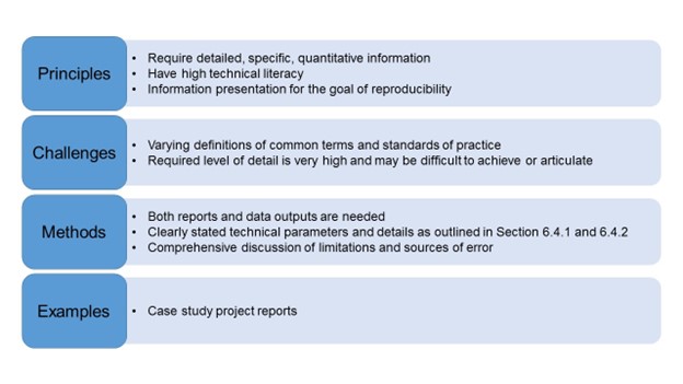
6.5.2 Risk Assessors

Those who assess risks due to coastal flood hazard are a key audience for flood risk information. Engineers and geoscientists (6.5.1) may be, and often are, also risk assessors. Risks are assessed for the purposes of planning infrastructure and communities, developing risk tolerance thresholds, informing insurance offerings, and informing mortgage and financial uptakes. Risk assessments are performed by professionals with a range of knowledge about technical aspects of coastal flood hazard management. The information in Figure 6.2 can be used to guide communicating the results of a coastal flood hazard assessment with risk assessors.

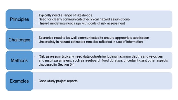
6.5.3 Emergency Managers

Emergency managers use coastal flood hazard information to inform mitigation, preparedness, response, and recovery. Findings may be used to support a number of initiatives including: pre-planning exercises, siting response resources, identification of potentially affected areas in response events, evacuation modelling, and prioritizing mitigations. Emergency managers use flood hazard information to inform plans, to communicate with the public, and to understand risks. While risk assessors often interpret coastal flood hazard information through risk assessments, emergency managers often also use coastal flood hazard information directly.

Emergency managers, more so than others, are often interested in worst-case scenarios, although they also need to understand the impact of a range of different events. When worst-case scenarios are considered, there is typically significant uncertainty associated with the modelling and significant implications of underestimating the hazards. Therefore, emergency managers may work with factors of safety and need these factors to be incorporated into hazard results. When evacuation routes are considered, emergency managers may need to understand the coastal flood hazard of an area outside of community or study boundaries to identify clear evacuation routes or refuge areas. While many emergency managers become well versed in the technical language of flood hazard analysis and mapping, clear definitions and non-technical language on maps are helpful for communicating results widely.

6.5.4 Land Use Planners and Approving Authorities

Planners play a vital role in reducing coastal flood risk through planning land use, communities, developments, and infrastructure. Approving authorities can include those with statutory decision-making authority over issues such as flood defences, site development permits, building permits, and bylaws governing lot filling. Planners work in short-, medium-, and long-term time horizons and need a clear understanding of change in risk over time. To effectively use coastal flood hazard and risk information, planners need a clear understanding of the relative risk of events, in order to tie these to community risk thresholds and associated land use or development plans. Clear communication to planners should include non-technical language, as well as full explanation of uncertainty and model limitations. As applicable, communicating with planners should include information about flood arrival times and extents, the impacts, extents and likelihoods of flooding over time, the effects of sea level rise, flood construction levels, factors of safety, and limitations of coastal defences.

6.5.5 Financial Planners

Financial planners can include banks, insurers, economists, and businesses (large and small). These agencies are looking to better understand the costs associated with disasters to support recovery and rebuilding in communities. Similar to emergency managers, financial agencies are looking to know where high-risk areas are located to inform financial planning decisions. The insurance industry typically works with catastrophe modellers to develop regional-scale models to understand coastal hazards and risks.

6.5.6 Public

The public uses coastal flood hazard information to understand their personal and their community’s risk. This can include real estate decisions, personal safety planning, and civic engagement on community risk. When developing information for the public, ensuring that the content is reviewed by or developed in part by the intended audience can help align the content appropriately with the audience.

When communicating to the general public, using a narrative approach that summarizes the detailed information and results in a story is recommended. A story used to communicate coastal flood hazard can have the following components:

• A beginning where coastal flood hazards are introduced in general.
• A middle where the results of the modelling are described depicting coastal flood hazards in the community.
• An end where the meaning of these coastal flood hazards for the community is described.

This narrative should read very differently from the detailed documentation of a technical report and focus instead on description of key aspects using audience-appropriate language.

6.5.7 Indigenous Nations

Many indigenous nations and people are at a greater risk of flooding. When communicating with Indigenous communities, having community-led conversations and information is invaluable to reflect the community’s context and sensitivities. For example:

• Use Indigenous place names on materials.
• Include Traditional Indigenous Knowledge.
• Consider reserve boundaries, territory boundaries, and potential contested land.

6.5.8 Other Audiences

Coastal flood hazard information is also used to understand risk by a variety of other audiences including the following:

• Politicians use it to inform themselves about issues of concern to their constituents and help develop policy direction and effective funding programs.
• Media are a key partner in sharing information and typically need clear narratives and visual resources to communicate effectively.
• Developers may use information to plan future projects and understand potential project risk at a high level before engaging in further planning and design
• Real estate professionals may reference information to guide their clients in purchasing properties. This is an increasing audience for flood hazard and risk information and efforts should be made to improve communication with this audience and consider industry impacts of new coastal hazard information.

When presenting information to any of these or other audiences, members of these groups should be involved in preparing or reviewing information as they will add the perspective of their discipline and ensure that the material is appropriate for the intended audience.

6.6 Other Communication Considerations

Sharing information from coastal flood hazard studies widely is essential to mobilizing information and effecting risk reduction. While there is some risk of misuse when sharing information, the benefits of disclosing information and sparking discussion typically outweigh the potential risks. Making information openly accessible is best practice for risk reduction and sharing information effectively requires consideration of the audience for the information.

Consideration should also be given to potential difficulties or liabilities associated with intellectual property and information disclosure. These should be considered from the outset of the project.

6.7 References

First Nations Information Governance Centre. (2014). First Nations Principles of OCAP®. https://fnigc.ca/ocap-training/

GoFair. (2016). FAIR principles. https://www.go-fair.org/fair-principles/

Greenan, B. J. W., James, T. S., Loder, J. W., Pepin, P., Azetsu-Scott, K., Ianson, D., Hamme, R. C., Gilbert, D., Tremblay, J.-E., Wang, X. L., & Perrie, W. (2018). Changes in oceans surrounding Canada; Chapter 7 in (eds.) Bush and Lemmen, Canada’s Changing Climate Report (pp. 343–423). Government of Canada.

Indigenous Advisory Sub-Committee on Indigenous Knowledge. (2020). Indigenous knowledge policy framework. Government of Canada. www.canada.ca/en/impact-assessment-agency/advisory/advisory-groups/indigenous-advisory-committee/principles-development-indigenous-knowledge-policy-framework.html

Intergovernmental Oceanographic Commission. (2019). Tsunami glossary. Intergovernmental Oceanographic Commission Technical Series. https://unesdoc.unesco.org/ark:/48223/pf0000188226.locale=en

Kim, J., Murphy, E., Nistor, I., Ferguson, S., & Provan, M. (2021). Numerical Analysis of Storm Surges on Canada’s Western Arctic Coastline. Journal of Marine Science and Engineering, 9(3), 326. https://doi.org/10.3390/jmse9030326

Murray, V., Abrahams, J., Abdallah, C., Ahmed, K., Angeles, L., Benouar, D., Brenes T., Alonso, C., Choe, Cox, S., Douris, J., Fagan, L., Fra Paleo, U., Han, Q., Handmer, J., Hodson, S., Khim, W., Mayner, L., Moody, N., Moraes, L., Osvaldo; Nagy, M., Norris, J., Peduzzi, P., Perwaiz, A., Peters, K., Radisch, J., Reichstein, M., Schneider, J., Smith, A., Souch, C., Stevance A., Triyanti, A., Weir, M., & Wright, N. (2021). Hazard information profiles: Supplement to UNDRR-ISC hazard definition & classification review: Technical report. United Nations Office for Disaster Risk Reduction, International Science Council. https://council.science/publications/hazard-information-profiles/ DOI: 10.24948/2021.05

NRCan. (2019). Federal geomatics guidelines for flood mapping. Federal Flood Mapping Guidelines Series. https://publications.gc.ca/collections/collection_2020/rncan-nrcan/m45/M45-114-2019-eng.pdf

NRCan (2024). Indigenous engagement guidelines for flood mapping. Government of Canada. https://natural-resources.canada.ca/science-and-data/science-and-research/natural-hazards/flood-mapping/federal-flood-mapping-guidelines-series/indigenous-engagement-guidelines-for-flood-mapping/26460

Shapiro, A. & Simpson, L. (1953). The effect of a broken ice field on water waves. Eos Transactions of the American Geophysical Union, 34, 36–42.