
Agriculture applications
The use of SAR imagery for agricultural applications has been studied extensively in particular because it is possible to acquire data at various times during the growing season. Single channel SAR data have been found to provide less information than multi-spectral optical data. This can be often overcome with a temporal series of SAR observations. As the crops grow and mature the backscatter characteristics change and these variations which depend on the crop can be used as the basis of crop discrimination.
The backscatter from agricultural targets is composed of surface scattering from the soil, volume scattering from the plants, and a soil-vegetation interaction term. The relative contribution of each component is a function of system and target parameters. In general, at C-band, the return is composed of a combination of these components with the soil surface term dominating early in the growing season and the vegetation volume term dominating during the peak growth period. At the end of the growing season, a mixture of the component returns is generally present with surface and soil-vegetation interaction terms being the dominant ones. This makes information extraction difficult as the soil or the crop may be the target of interest and other components produce "noise" which adds significant error to the estimation process. Once again multi-temporal observations help, but difficulties persist.
Research to date has demonstrated that the additional information in polarimetric data (both magnitude and phase) can help to increase the information content for agricultural applications thereby decreasing the need for multi-temporal imagery.
Crop productivity/within field variation
Crop productivity depends on numerous factors including soil characteristics, climatic variables and crop management practices. Crop biomass, green leaf area and green leaf duration are indicators of crop condition and potential yield.. The extent to which biomass and Leaf Area Index (LAI), can be effectively monitored using microwave imagery is an ongoing area of research. The sensitivity of SAR data to crop condition is a function of imaging parameters such as wavelength, incidence angles and polarization, as well as parameters such as crop type and phenological stage (e.g. size, distribution, orientation and dielectric properties of component parts of the canopy).
In the following, two examples of the use of polarimetric data for crop condition monitoring are presented (from the work of McNairn et al.  ):
):
- the use of imagery in multiple polarizations to separate regions in a field with variations in crop condition.
- the ability to discern scattering mechanisms associated with zones of crop condition variability using the H/A/
 algorithm developed by Cloude and Pottier .
9.1.3.1 Within Field Variation as related to Polarization
The ability to determine variations within a field is illustrated using polarimetric C-SAR data acquired over Southen Ontario on June 30, 1999 as described by McNairn et al. . Imaging polarization combinations examined included the four linear transmit-receive polarizations (HH, VV, HV, and VH), as well as two circular transmit-receive polarizations (RR and LR).
A winter wheat field is used to illustrate the mapping of in-field variations(Figure 9-6a). A simple RGB image (R=VV, G=HV, B=HH) shows regions of low backscatter. Yield monitor data obtained two weeks following the SAR acquisition showed that these low backscatter areas corresponded to yields less than 70 bushels per acre (BPA).
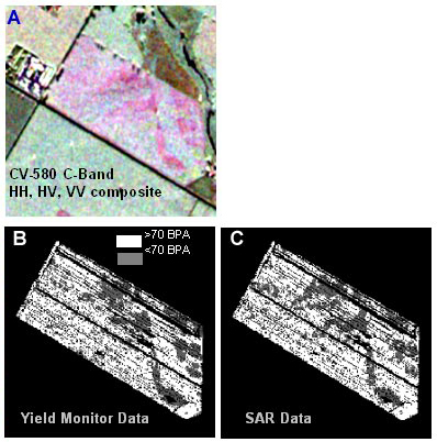
Figure 9-6. a) C-band image of winter wheat image (R=VV, G=HV, B=HH ); b) classified yield monitor data, bushels per acre (BPA), c) classified SAR data differentiating low and high yield zones (Noetix Research Inc., 2001)
It is noted that imagery at C-Band in HH alone could not have been used to separate the zones of different productivity. (Figure 9-7). Imagery in the linear cross-polarization (HV) was found to show the greatest contrast between the higher and lower productivity zones (4.1 dB), and this was followed by imagery in VV, RR, and LR polarizations showing differences of approximately 2 dB.
Figure 9-7. Backscatter at linear and circular polarizations for lower and higher producing zones of white winter wheat (from ).
The areas of low yield within the wheat field identified using the three linear polarizations agreed reasonably (77%) with the low yield areas identified by the yield monitor data.
A) Area of Agreement (Higher Yield) 77%
B) Area of Agreement (Lower Yield) 77%
C) "Error" (omission/comission) 23%
Figure 9-8. Percent agreement between SAR classification and yield monitor data .
Scattering mechanisms and within-field variation
Relating backscatter values to crop condition is not always straight forward. An area of high biomass within a wheat field for example, may have lower backscatter or a higher backscatter relative to an area of lower biomass depending on the phenological stage of a crop and/or environmental conditions (including background soil moisture) at the time of image acquisition. For example, in a wheat field with high volumetric soil moisture, low biomass areas will have higher backscatter than the high biomass area. The opposite can be true given low volumetric soil moisture.
Polarimetric classification algorithms such as those based on Cloude and Pottier's H/A/ can be used to identify the scattering mechanism and thus help in the interpretation of the observed backscatter.
Polarimetric C-SAR data were collected near Indianhead, SK using the CV-580 platform. Several polarizations were synthesized from the complex data. The polarizations used in the unsupervised classification including HH, VV, HV, RR, RL and linear polarizations with 45° and 135° orientations. The resulting map created 6 productivity zones over three crop types (Figure 9-9).
In one study performed by McNairn et al. polarimetric C-SAR data were collected near Indian Head, SK in June 2000. Several polarizations were synthesized from the complex data, including two circular polarizations (RR and RL). Linear polarizations were synthesized by choosing an ellipticity angle ( ) of zero and by varying the orientation angle (
 ) at 45° increments from 0° to 180°. Incidence angles over the test site were between 42° and 46°. The SAR image was classified into sixteen clusters using seven of these polarizations as input and a K-Means algorithm (Figure 9.9). The polarizations used in the unsupervised classification included HH, VV, HV, RR, RL and linear polarizations with = 45° and = 135°. These seven images were used as input to classify the wheat crops into six classes representing three growth zones: very healthy growth (zone 1); average growth (zone 2); poor growth (zone 3).
Figure 9-9. Productivity zones generated from an unsupervised classification of images for HH, VV, HV, RR, RL and linear polarizations with  = 45° and = 135° for wheat (1), canola (2) and peas (3), June 28, 2000 .
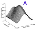
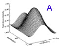
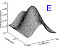
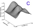
The three growth zones representing high to low biomass for the wheat fields were used as a mask to extract the H/ parameters of Cloude and Pottier. The H/ plane for a high biomass site is presented in Figure 9-10. In general, regions 1, 4, and 7 identify regions dominated by multiple scattering, regions 2, 5,and 8 dominated by volume scattering, and regions 3, 6, and 9 by surface scattering.
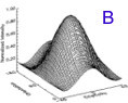
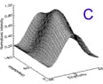
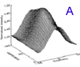
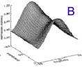
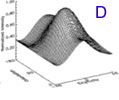
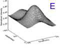
Figure 9-10 suggests that the backscatter from high biomass wheat is dominated by volume scattering. Figure 9-11 was derived from the zone of average growth and again, volume scattering by the canopy is the dominant mechanism. In Figure 9-12 the zone of poor growth, where crop biomass is low, is dominated by surface scattering [McNairn, Personal Communication].
Area 24: wheat Line 0 Pass 0 0
Cloude Alpha ( ) vs Entropy (H) - Density Histogram
A = Multiple Scattering B = Volume Scattering C = Surface Scattering
D = Low Entropy E = Medium Entropy F = High Entropy
| Entropy | Anisotropy | |
 |
|
|---|---|---|---|---|
| Average | 0.81 | 0.43 | 42.04 | 17.51 |
| Standard Deviation | 0.03 | 0.07 | 2.65 | 2.89 |
Figure 9-10. H / plane with bounds and partitioning showing a high biomass area within the wheat field
Area 48: wheat Line 0 Pass 0 0
Cloude Alpha () vs Entropy (H) - Density Histogram
A = Multiple Scattering B = Volume Scattering C = Surface Scattering
D = Low Entropy E = Medium Entropy F = High Entropy
| Entropy | Anisotropy | |
|
|
|---|---|---|---|---|
| Average | 0.75 | 0.53 | 41.34 | 16.39 |
| Standard Deviation | 0.03 | 0.06 | 1.76 | 3.19 |
Figure 9-11. Scattering as shown in the H/ plane for a medium biomass area within the spring wheat field.
Area 13: wheat Line 0 Pass 0 0
Cloude Alpha () vs Entropy (H) - Density Histogram
A = Multiple Scattering B = Volume Scattering C = Surface Scattering
D = Low Entropy E = Medium Entropy F = High Entropy
| Entropy | Anisotropy | |
|
|
|---|---|---|---|---|
| Average | 0.74 | 0.44 | 35.52 | 15.27 |
| Standard Deviation | 0.04 | 0.06 | 3.45 | 2.99 |
Figure 9-12. Scattering as shown in the H/ plane for a low biomass area within the spring wheat field.
Soil conservation: soil tillage and crop residue
Soil conservation is a major concern in agriculture. Tillage practices have direct bearing on the potential for wind and water erosion, and soil quality, especially as it relates to the maintenance of soil organic matter. The ability to monitor the type of tillage, and amount of residue is important for soil conservation. Tillage affects surface roughness (as a function of implements used and number of passes) and the amount of residue , , . Due to the sensitivity of radar backscatter to field characteristics including surface roughness, polarimetric data may prove very useful for monitoring soil tillage and crop residue.
There are a number of polarimetric parameters found to be useful for discriminating soil tillage/residue. Highlighted here are the use of Co-polarization Signatures and Co-polarization Phase Difference.
9.1.2.1 Polarimetric Signatures
Polarization signatures are a graphical method of visualizing the backscatter response of a target as a function of incident and backscattered polarizations. Polarization signatures can be used to give a graphical presentation of the backscattering characteristics and can therefore be useful in differentiating target characteristics. In this example, this is shown in relation to variations in tillage and residue cover.
Co-polarization plots were obtained from SIR-C imagery for fields with varying tillage and amounts and types of residue in a study by McNairn et al.
A) Tilled Field with Little or No Residue
The following co-polarization plots were obtained from C-band (Figure 9-1) and L-band (Figure 9-2) imagery for tilled fields with varying amounts and types of residue. Incidence angles were between approximately 42 and 50 degrees .
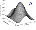
 A) Pea Residue (25% residue cover) |
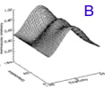
 B) Lentil Residue (25% residue cover) |
 C) Canola Residue (40% residue cover) |
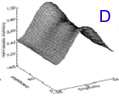
 D) Wheat/Barley Residue (20% residue cover) |
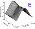
 E) Sunflower Residue (40% residue cover) |
|
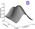
| Figure 9-1. C - Band co-polarization signatures, tilled field with little or no residue (from ). |
||
The smoothest fields, those with the finest residue have a maximum response at VV polarization (Orientation Angle of 90°). Backscatter was approximately equal at all linear polarizations for the canola, wheat/barley and sunflower residue fields, suggesting that these fields appear rougher.
 A) Pea Residue (25% residue cover) |
 B) Lentil Residue (25% residue cover) |
 C) Canola Residue (40% residue cover) |
 D) Wheat/Barley Residue (20% residue cover) |
 E) Sunflower Residue (40% residue cover) |
|
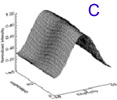
| Figure 9-2. L-Band co-polarization signatures, tilled field with little or no residue.(from ). |
||
In the L-Band example, fields that had been tilled or had very fine residue cover exhibited responses typical of surface scattering. For these targets, maximum response is at an Orientation Angle of 90° and the target appears flat relative to the wavelength. For these fields, the low pedestal heights(0.18-0.24) indicate minimal depolarisation, hence confirm that surface scattering is dominant. These surfaces are not rough enough and do not have enough vegetative material to cause significant multiple or volume scattering. The difference between VV and HH backscatter is much more pronounced at L-Band than at C-Band, since at this longer wavelength, these surfaces appear much smoother.
B. No-Till Residue Fields with Multiple Scattering
The following co-polarization plots were obtained from C-band (Figure 9-3) and L-band (Figure 9-4) imagery for no-till fields with varying amounts and types of residue. (from )
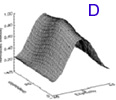
Plots for C-Band (Figure 9-3) with the exception of (a) exhibit a saddle type shape typical of double bounce scattering. The pedestal height in these co-polarization plots was larger and thus indicates that greater depolarization was occurring on the no-till fields as compared to the tilled fields with low residue cover. The pea residue field (Figure 9-3a) shows a response similar to that for the field with pea residue that had been tilled (Figure 9-1a). Comparison of these two figures suggests that very fine residue has little effect on radar response as this target appears "smooth" at C-Band.
 A) Pea Residue |
 B) Lentil Residue |
 C) Canola Residue |
 D) Wheat/Barley Residue |
 E) Sunflower Residue |
|
| Figure 9-3. C-Band co-polarization signatures, no till fields with multiple scattering.(from ). |
||
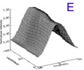
The co-polarization plots for L-Band imagery are significantly different when compared to those at C-Band. Relative to C-band the double bounce scattering is substantially reduced with a VV peak often present, indicating significant surface scattering for wheat/barley, and sunflower residues.
 A) Pea Residue |
 B) Lentil Residue |
 C) Canola Residue |
 D) Wheat/Barley Residue |
 E) Sunflower Residue |
|
| Figure 9.4. L-Band co-polarization signatures, no till fields with multiple scattering (from ). |
||
A full discussion of polarimetric plots and other polarimetric parameters related to differentiating tillage and field residue is given in McNairn et al
9.1.2.2 Co-Pol Phase Difference (PPD)
The Co-polarization Phase Difference is a polarimetric parameter that may be useful for characterizing backscattering mechanisms. For instance, a single bounce (or odd bounce) scatterer will have a relative phase difference between HH and VV of 0° in the FSA For a double bounce (or even bounce) scatterer, the phase difference will be 180°. If the basis convention is changed to the BSA there is a further sign change, which adds 180° to the phase difference. As an example, bare soils are surface scatterers, and generally have a mean Co-polarized Phase Difference equal to 0° with a small standard deviation.
Ulaby et al. suggested that much of the information content provided by the Co-polarized Phase Differences lies in the distribution of these differences (as expressed by the standard deviation) e.g., a rough plowed field has a phase distribution that is broad when compared to that for a smoother disked field.
As shown in the study by McNairn et al. , the Mean Co-polarized Phase Difference was found to be close to zero for most fields with residue and so provided little useful information . Standing senesced crops did show phase differences significantly greater than 0° with the mean phase differences varying between the fields where multiple scattering is believed to occur. In terms of tillage practices, mean phase differences for fields could not be used to distinguish between the presence or absence of tillage and residue types, although differences were found between standing senesced crops and harvested fields. For example, the standing senesced corn and sunflower fields tended to have much higher mean phase differences varying between -30° and -130° for C-Band and -30° and -90° for L-Band. The field based phase distribution data can be used to differentiate tilled low residue fields from no-till (high residue) fields. The standard deviation of the phase differences for fields with low residue cover was less than 30o; the standard deviation for no-till fields exceeded 45°. These results are consistent with those reported by Ulaby et al. . An example figure showing the distribution of fields with various Mean Phase Differences is given as Figure 9.5 (modified from ).
Figure 9-5. C-Band field based co-polarized phase distribution does vary as a function of residue characteristics (modified from McNairn et al. ).
Whiz quiz
 Question: How would the polarization phase difference (PPD) compare for a bare field and a standing corn field?
Whiz quiz - answer
Answer: The PPD would have a mean close to zero with a small standard deviation for the bare field. The corn field would have a mean PPD different from zero with a larger standard deviation.
Page details
- Date modified: