Polarimetric Image Interpretation

One of the main objectives of remote sensing is to make a thematic map of the Earth's surface, indicating the type of material at each location imaged by the radar. The type of material can be estimated from the polarimetric radar data, using a computer-based classification algorithm. Pixels or groups of pixels are assigned to terrain classes that have a meaningful geoscientific interpretation.

In the case of polarimetric radar, a larger number of parameters can be measured compared to a single-channel radar. This should make it possible to achieve a more accurate image classification. However, measurement noise, system calibration difficulties, the understanding of scattering mechanisms and the mixing of many different scattering mechanisms in one pixel or group of pixels are obstacles that must be overcome to obtain an accurate classification. The issues of calibration and image interpretation are addressed in this section. Details of classification algorithms are given in Section 7.

Data calibration

One of the critical requirements of polarimetric radar systems is the need for calibration. This is because much of the information lies in the ratios of amplitudes and the differences in phase angle between the backscattering in the four received polarization combinations. If the calibration is not sufficiently accurate, the scattering mechanisms will be misinterpreted and the advantages of using multiple polarizations will be lost.

Calibration is achieved by a combination of radar system design and analysis of the received data. Consider the response to a trihedral corner reflector shown in Figure 6-1. This ideal response is represented by the identity scattering matrix:
     
and is only obtained if the four channels all have the same gain, the phase differences between channels are corrected to zero, there is no energy leakage from one channel to another (crosstalk), and there is no receiver noise. Even if the radar system does not have these ideal properties, if the imbalances can be measured, they can be largely corrected by calibration procedures.

In terms of the radar design, the channel gains and phases should be as carefully matched as possible. In the case of the phase balance, this means that the signal path lengths should be effectively the same in all channels. Calibration signals are usually built into the system design to measure the channel balances.

In terms of data analysis, channel balances (amplitude and phase), crosstalk and noise can be measured and corrected by analyzing the data received from specific targets. In addition to analyzing the response of internal calibration signals, the signals from known targets such as corner reflectors, active transponders, uniform clutter and radar shadow can be used to calibrate some of the parameters.

Many different calibration procedures have been developed, some sensor-specific , , , , , , , . One of the common difficulties is that the calibration parameters tend to vary with beam elevation angle (because of antenna properties) and with incidence angle (because of scattering properties), which means that the calibration procedure has to account for range variations in the scene.

In addition to compensating for system imbalances, there are the calibration issues of interpreting absolute gain values, and the geometric location of the processed samples. Traditionally, corner reflectors and active radar calibrators (ARCs) are deployed on the ground for these purposes. For geometric location, a simple, economical wire mesh reflector can be used (see Figure 6-1). But for precise gain measurement, a corner reflector with close structural tolerances or an ARC are generally used (see Figure 6-2).

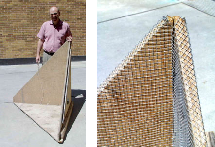
Figure 6-1: A wire mesh 1.4 meter corner reflector used for geometric calibration. The internal surfaces meet at 90°, and are covered by a conducting mesh to create a strong backscatter. CCRS calibration specialist, Bob Hawkins is the proud father.

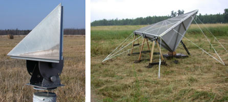
Figure 6-2: Small (40 cm) and large (140 cm) trihedral corner reflectors used by CCRS for radar calibration. Larger reflectors are needed at lower frequencies, as the reflector gain is proportional to the square of the radar frequency. (source: CCRS)

Interpretation based on scattering models

The next higher level of complexity involves an understanding of the scattering mechanisms present. Van Zyl introduced an unsupervised classifier in which image pixels are assigned to classes of "odd bounce", "even bounce" and "diffuse" scattering mechanisms . This is based upon the principle that scatterers of simple geometrical structure have primarily a co-pol response, but the number of bounces or reflections that the radar signal experiences creates a recognizable phase difference between the HH and the VV channels (the relative phase changes by 180° for every bounce). Van Zyl developed a simple mathematical test to separate each pixel into these three classes .

Another set of scattering models based on physical principles was introduced by Freeman and Durden . Taking a tree on rough ground as a generic scatterer, the radar energy backscattered by the canopy, the trunk and the ground are modelled and used to categorize naturally occurring scatterers. A mathematical procedure was developed that computed the percentage of each type of scatterer in each pixel. The method is similar to that of van Zyl, except that a physical model is used to separate scattering mechanisms in the data, rather than a purely mathematical rule.

When faced with a large number of measured parameters, classifiers work better if the parameter set can be transformed into an orthogonal set, and the dimensionality of the set reduced to those parameters containing meaningful information (i.e. removing noisy parameters). Eigenvalue methods can be used to advantage, and it is helpful to use scattering models that are independent of the scene content. One of the latest methods of parameter selection is based on an eigenvalue decomposition of the coherency matrix developed by Cloude and Pottier Cloude decomposition), where the parameters of polarimetric entropy, polarimetric anisotropy and alpha angle are calculated from the eigenvalues and eigenvectors of the matrix.

Entropy (H) represents the randomness of the scattering, with H = 0 indicating a single scattering mechanism and H = 1 representing a random mixture of scattering mechanisms, i.e. a depolarizing target. Values in between indicate the degree of dominance of one particular scatterer. The angle is based upon the eigenvectors and is a number indicative of the average or dominant scattering mechanism. The lower limit of = 0° indicates surface scattering, = 45° indicates dipole or volume scattering, while the upper limit of = 90° represents a dihedral reflector or multiple scattering. Another parameter that provides useful scattering information is anisotropy, a parameter based upon the ratio of eigenvalues, which indicates multiple scatterers.

Visual interpretation

The simplest classification method is performed by visual interpretation. An interpreter learns how surface features are portrayed in the image, and his/her mind fills in missing details based upon local knowledge and experience.

To aid visual interpretation, the multiple channels of polarimetric data can be used to present the data in a colour image, in which certain image features are recognizable by a trained interpreter. As a simple example, a colour image can be made using an HH=red, HV=green and VV=blue channel assignment (see Figure 6-3). This tends to "look realistic" as water reflections have a higher VV component than HH, and vegetation has a higher than average HV backscatter.

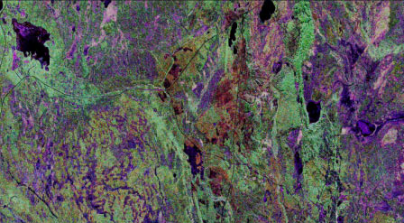
Figure 6-3: SIR-C L-band colour composite image of Nipawin Provincial Park, north of Prince Albert, Saskatchewan (HH - red, HV - green and VV - blue)

As an example of the interpretation that can be obtained from such an image, the following description is from the NASA web site: http://visibleearth.nasa.gov/. Search: Space Radar Image of Prince Albert, Canada

This is a false-color composite of Prince Albert, Canada, centered at 53.91 north latitude and 104.69 west longitude. This image was acquired by the Spaceborne Imaging Radar C/X-Band Synthetic Aperture Radar (SIR-C/X-SAR) aboard space shuttle Endeavor on its 20th orbit. The area is located 40 kilometers (25 miles) north and 30 kilometers (20 miles) east of the town of Prince Albert in the Saskatchewan province of Canada. The image covers the area east of the Candle Lake, between gravel surface highways 120 and 106 and west of 106. The area in the middle of the image covers the entire Nipawin (Narrow Hills) provincial park. The look angle of the radar is 30 degrees and the size of the image is approximately 20 kilometers by 50 kilometers.

The image was produced by using only the L-band. The three polarization channels HH, HV and VV are illustrated by red, green and blue respectively. The changes in the intensity of each color are related to various surface conditions such as variations in forest stands, frozen or thawed condition of the surface, disturbances (fire and deforestation), and areas of regrowth. Most of the dark areas in the image are the ice-covered lakes in the region. The dark area on the top left corner of the image is the White Gull Lake north of the intersection of highway 120 and 913. The right middle part of the image shows Lake Ispuchaw and Lower Fishing Lake. The deforested areas are also shown by dark areas in the image. Since most of the logging practice at the Prince Albert area is around the major highways, the deforested areas can be easily detected as small geometrically shaped dark regions along the roads.

At the time of the SIR-C/X-SAR overpass a major part of the forest is either frozen or undergoing the spring thaw. The L-band HH shows a high return in the jack pine forest. The reddish areas in the image are old jack pine forest, 12 to 17 meters in height and 60 to 75 years old. The orange-greenish areas are young jack pine trees, 3 to 5 meters (10 to 16 feet) in height and 11 to 16 years old. The green areas are due to the relative high intensity of the HV channel, which is strongly correlated with the amount of biomass. The L-band HV channel shows the biomass variations over the entire region. Most of the green areas, when compared to the forest cover maps are identified as black spruce trees. The dark blue and dark purple colors show recently harvested or regrowth areas respectively.